Now wearing my “ops” hat, there are a few things that I wanted to cover - blocking bad clients, rate limiting, caching, and gradual rollout.

Blocking bad clients

Blocking bad clients in nginx is usually implemented with a simple return 403 for some requests. To classify request we can use any builtin variable, e.g. $http_user_agent to match by user agent:

server {
    # ...

    # Block all bots
    if ($http_user_agent ~ ".*bot.*") {
        return 403;
    }

    # ...
}

If you need more conditions to identify bad clients, use the map to construct the final variable like this:

http {
    # Ban bots using specific API key
    map $http_user_agent:$arg_key $ban {
        ~.*bot.*:1234567890 1;
        default 0;
    }

    server {
    # ...

        if ($ban = 1) {
            return 403;
        }

    # ...
    }
}

Simple and easy. Now, let’s see more involved cases where we need to rate limit some clients.

Rate limiting

Rate limiting allows you to throttle requests by some pattern. In nginx it is configured with 2 directives:

1. limit_req_zone where you describe the “zone”. A zone contains configuration on how to classify requests for rate limiting and the actual limits.
2. limit_req that applies zone to the particular context - http for global limits, server per virtual server, and location for a particular location in a virtual server.

To illustrate this, let’s say we need to implement the following rate limiting configuration:

• Global rate limit of 100 RPS by IP
• Limit search engine crawlers to 1 RPM. Crawlers are determined by the User-Agent header.
• Limit requests from some bad client by API token to 1 RPS.

To classify requests you need to provide a key to the limit_req_zone. key is usually some variable, either predefined by nginx or configured by you via map. All requests that share some key value will be tracked in that hash table for rate limiting.

To setup the global rate limit by IP, we need to provide IP as a key in limit_req_zone. Looking at varindex for predefined variables you can see the binary_remote_addr that we will use like this:

http {
    # ...
    limit_req_zone $binary_remote_addr zone=global:100m rate=100r/s;
    # ...
}

Heads up: if your nginx is not public, i.e. it’s behind another proxy, the remote address will be incorrectly attributed to the proxy before your nginx. Use the set_real_ip_from directive to extract the remote address of the real client from request headers.

Now, to limit search engine crawlers by User-Agent header we have to use map:

http {
    # ...
    map $http_user_agent $crawler {
        ~*.*(bot|spider|slurp).* $http_user_agent;
        default "";
    }

    limit_req_zone $crawler zone=crawlers:1M rate=1r/m;
    # ...
}

Here we are setting $crawler variable as a limit_req_zone key. The key in limit_req_zone must have distinct values for different clients to correctly attribute request counters. We store the real user agent value for keys, so all requests with a particular user agent will be accounted as a single stream regardless of other properties like IP address. If the request is not from a crawler we use an empty string which disables rate limiting.

Finally, to limit requests by API token we use map to create a key variable for another rate limit zone:

http {
    # ...
    map $http_authorization $badclients {
        ~.*6d96270004515a0486bb7f76196a72b40c55a47f.* 6d96270004515a0486bb7f76196a72b40c55a47f;
        ~.*956f7fd1ae68fecb2b32186415a49c316f769d75.* 956f7fd1ae68fecb2b32186415a49c316f769d75;
        default "";
    }
    # ...
    limit_req_zone $badclients zone=badclients:1M rate=1r/s;
}

Here we look into the Authorization header for API token like Authorization: Bearer 1234567890. If we matched against a few known tokens we use that value for $badclients variable and then again use it as a key for limit_req_zone.

Now, that we have configured 3 rate limit zones we can apply them where it’s needed. Here is the full config:

http {
    # ...
    # Global rate limit per IP.
    # Used when child context doesn't provide rate limiting configuration.
    limit_req_zone $binary_remote_addr zone=global:100m rate=100r/s;
    limit_req zone=global;
    # ...

    # Rate limit zone for crawlers
    map $http_user_agent $crawler {
        ~*.*(bot|spider|slurp).* $http_user_agent;
        default "";
    }
    limit_req_zone $crawler zone=crawlers:1M rate=1r/m;

    # Rate limit zone for bad clients
    map $http_authorization $badclients {
        ~.*6d96270004515a0486bb7f76196a72b40c55a47f.* 6d96270004515a0486bb7f76196a72b40c55a47f;
        ~.*956f7fd1ae68fecb2b32186415a49c316f769d75.* 956f7fd1ae68fecb2b32186415a49c316f769d75;
        default "";
    }
    limit_req_zone $badclients zone=badclients:1M rate=1r/s;

    server {
        listen 80;
        server_name www.example.com;
        # ...
        limit_req zone=crawlers; # Apply to all locations within www.example.com
        limit_req zone=global; # Fallback
        # ...
    }

    server {
        listen 80;
        server_name api.example.com;
        # ...
        location /heavy/method {
            # ...
            limit_req zone=badclients; # Apply to a single location serving some heavy method
            limit_req zone=global; # Fallback
            # ...
        }
        # ...
    }

}

Note that we had to add global zone as a fallback whenever we have other limit_req configurations. That’s needed because nginx fallback to limit_req defined in the parent context only if the current context doesn’t have any limit_req configuration.

So the general pattern for configuring rate limiting is the following:

• Prepare variable that will store a key for rate limiting. The keys must be distinct for different rate limiting buckets.
• Empty key disables rate limiting.
• Use the variable with rate limiting key to configure rate limiting zone configuration.
• Apply rate limit zone where needed with limit_req.
• If you need a fallback configuration, define it together with the configuration on the current level.

Rate limit will help to keep your system stable. Now let’s talk about caching that can remove some excessive load from the backends.

Caching

One of the greatest features of nginx is its ability to cache responses.

Let’s say we are proxying requests to some backend that returns static data that is expensive to compute. We can shave the load from that backend by caching its response.

Here is how it’s done:

http {
    # ...
    proxy_cache_path  /var/cache/nginx/billing keys_zone=billing:500m max_size=1000m inactive=1d;
    # ...

    server {
        # ...
        location /billing {
            proxy_pass http://billing_backend/;

            # Apply the billing cache zone
            proxy_cache billing;

            # Override default cache key. Include `Customer-Token` header to distinguish cache values per customer
            proxy_cache_key "$scheme$proxy_host$request_uri $http_customer_token";

            proxy_cache_valid 200 302 1d;
            proxy_cache_valid 404 400 10m;
        }
    }
}

In this example, we cache responses from the “billing” service that returns billing information for a client. Imagine that these requests are heavy so we cache them per customer. We assume that clients access our billing API with the same URL but provides a Customer-Token HTTP header to distinguish themselves.

First, caching needs some place where it will store the values. This is configured with the proxy_cache_path directive. It needs at least 2 required params - keys_zone and path. The keys_zone gives a name to the cache and sets the size of the hash table to track cache keys. Path will hold the actual files named after MD5 hash of the cache key which is, by default, is the full URL of the request. But you can, of course, configure your own cache key with the proxy_cache_key directive where you can use any variables including HTTP headers and cookies.

In our case, we have overridden the default cache key by adding the $http_customer_token variable holding the value of the Customer-Token HTTP header. This way we will not poison the cache between customers.

Then, as with rate limits, you have to apply the configured cache zone to the server, location, or globally using proxy_cache directive. In my example, I’ve applied caching for a single location.

Another important thing to configure from the start is cache invalidation. By default, only responses with 200, 301, and 302 HTTP codes are cached, and values older than 10 minutes will be deleted.

Finally, when proxying requests to upstreams, nginx respects some headers like Cache-Control. If that header contains something like no-store, must-revalidate then nginx will not cache the response. To override this behavior add proxy_ignore_headers "Cache-Control";.

So to configure nginx cache invalidation do the following:

• Set the max_size in proxy_cache_path to bound the amount of disk that cache will occupy. If the nginx would need to cache more than max_size it will evict the least recently used values from the cache
• Set the inactive param in proxy_cache_path to configure the TTL for the whole cache zone. You can override it with proxy_cache_valid directive.
• Finally, add proxy_cache_valid directive that will instruct the TTL for the cache items in a given location or server and that will set TTL for cache items.

In my example, I’ve configured caching of 200 and 302 responses for a day. And also for error responses I’ve added caching for 10 minutes to avoid thrashing the backend in vain.

Gradual rollout of a new service

Another feature that is rarely used, but when it’s needed it’s a godsend, is a gradual rollout.

Imagine you are doing a massive rewrite of your product. Maybe you’re migrating to a new database system, rewriting backend in Go, or moving to a cloud. Whatever.

Your current version is used by all of the clients and you have deployed the new version alongside. How would switch clients from the current backend to the new one? The obvious choice is to just flip the switch and hope everything will work. But hope is not a good strategy.

You could’ve tested your new version rigorously. You might even do the traffic mirroring to ensure that your new system operates correctly. But anyway, from my experience there is always something that goes wrong - forgotten important header in the response, slightly changed format, rare request that swamps your DB.

I’m sure that it’s better to gradually rollout massive changes. Even a few days helps a lot. Sure, it requires more work to do but it pays off.

The main feature in nginx that provides gradual rollout is a split_client module. It works like map but instead of setting variable by some pattern, it creates the variable from the source variable distribution. Let me illustrate it:

http {
    upstream current {
        server backend1;
        server backend2;
    }

    upstream new {
        server newone.team.svc max_fails=0;
    }

    split_clients $arg_key $destination {
        5% new;
        *  current;
    }

    server {
        # ...
        location /api {
            proxy_pass http://$destination/;
        }
    }
}

This split_client configuration does the following - it looks into the key query argument and for 5% of the values it sets $new_backend to 1. For the other 95% of keys, it will set $new_backend to 0. The way it works is that the source variable is hashed into a 32-bit hash that produces values from 0 to 4294967296, and the X percent is simply the first 4294967296 * X / 100 values (for 5% it’s a 4294967296 * 5 / 100 = 214748364 first values).

Just to give you a sense of how the 5% example above behaves, here is what distribution looks like

key | $destination
----+-------------
1   |   current
2   |   current
3   |   current
4   |   current
5   |   current
6   |   current
7   |   current
8   |   new
9   |   current
10  |   new

Since split_client creates a variable you can use it in our beloved map to construct more complex examples like this:

http {
    upstream current {
        server http://backend1/;
        server http://backend2/;
    }

    upstream new {
        server http://newone.team.svc/ max_fails=0;
    }

    split_clients $arg_key $new_api {
        5% 1;
        *  0;
    }

    map $new_api:$cookie_app_switch $destination {
        ~.*:1 new;
        ~0:.* current;
        ~1:.* new;
    }

    server {
        # ...
        location /api {
            proxy_pass http://$destination/;
        }
    }
}

In this example, we are combining the value from the split_clients distribution with the value of the app_switch cookie. If the cookie is set to 1, we set $destination to new upstream. Otherwise, we look into the value from split_clients. This is a kind of feature flag to test the new system in production - everyone with the cookie set will always get responses from the new upstream.

The distribution of the keys is consistent. If you’ve used API key for split_clients then the user with the same API key will always be placed into the same group.

With this configuration, you can diverge traffic to the new system starting with some small percentage and gradually increment the percentage. The little downside here is that you have to change the percentage value in the config and reload nginx with nginx -s reload to apply it - there is no builtin API for that.

Now, let’s talk about nginx logging.

Structured logs

Collecting logs from nginx is a great idea because it’s usually an entrypoint for the clients’ traffic and so it can report actual service experience as customers see it.

To get any profit from logs they should be collected in some central place like Elastic stack or Splunk where you can easily query and even build decent analytics from it. These log management tools require structured data but nginx by default is logging in the so-called “combined” log format which is an unstructured mess that is expensive to parse.

The solution to this is simple - configure structured logging for nginx. We can do this with the log_format directive. I always log in JSON format because it’s understood universally. Here is how to configure JSON logging for nginx:

http {
    # ...
    log_format json escape=json '{'
        '"server_name": "billing-proxy",'
        '"ts":"$time_iso8601",'
        '"remote_addr":"$remote_addr","host":"$host","origin":"$http_origin","url":"$request_uri",'
        '"request_id":"$request_id","upstream":"$upstream_addr",'
        '"response_size":"$body_bytes_sent","upstream_response_time":"$upstream_response_time","request_time":"$request_time",'
        '"status":"$status"'
        '}';
    # ...
}

Yes, it’s not the prettiest thing in the world but it does the job. You can use any variables in the format - builtin in nginx and your own that you defined with the map directive.

I use implicit string concatenation here to make it more readable - there are multiple single-quoted strings one after another that nginx will glue together. Inside each string, I use double-quoted strings for JSON fields and values.

The escape=json option will replace non-printable chars like newlines with escaped values, e.g. \n. Quotes and backslash will be escaped too.

With this log format, you don’t need to use the grok filter in logstash and painfully parse logs into some structure. If nginx is running in kubernetes all you have to do is:

filter {
    json {
        source => "log"
        remove_field => ["log"]
    }
}

Because logs from containers are wrapped in the JSON where the log message is store in the "log" field)

Conclusion

And that’s a wrap for my nginx experience so far. I’ve written about nginx mirroring, shared a few features useful when you develop backends behind nginx and here I’m dumping the rest of my knowledge gained while using nginx in production.

First, let’s look at the simple config that just forwards requests from http://proxy.local/ address to a single http://backend.local:10000.

user nginx;
worker_processes auto;

events {}

http {
    access_log  /var/log/nginx/access.log combined;

    # include /etc/nginx/conf.d/*.conf;

    upstream backend {
        server backend.local:10000;
    }

    server {
        server_name proxy.local;
        listen 8000;

        location / {
            proxy_pass http://backend;
        }
    }
}

You declare your backend service as an upstream group. Each instance of the backend is described with a server directive.

Then you declare entrypoint with a server and location. Given that it’s nginx you can go crazy with regexp location matching and stuff but it’s not what is required in the case of service routing.

Finally, you forward requests with proxy_pass directive.

From this simple config, we can start to build the necessary complexity.

Active/Passive backend configuration

If your service needs active/passive configuration where one server is the main for requests handling and the other is a backup then you can configure it like this:

    ...
    upstream backend {
        server main-backend.local:10000;
        server backup-backend.local:10000 backup;
    }
    ...    

backup option tells nginx that this server in the upstream group will be used only if the primary server is unavailable.

By default, server is marked as unavailable after 1 connection error or timeout. This can be tuned with max_fails option for each server in an upstream group like this:

    ...
    upstream backend {
        # Try 3 times for the main server
        server main-backend.local:10000 max_fails=3;

        # Try 10 times for backup server
        server backup-backend.local:10000 backup max_fails=10;
    }
    ...    

In addition to connection errors and timeouts, you can use various HTTP error codes like 500 as unsuccessful attempts. This is configured by the proxy_next_upstream directive.

...
    upstream backend {
        server main-backend.local:10000;
        server backup-backend.local:10000 backup;
    }

    server {
        server_name proxy.local;
        listen 8000;

        # Switch to the next upstream in  case of connection error, timeout
        # or HTTP 429 error (rate limit).
        proxy_next_upstream error timeout http_429;

        location / {
            proxy_pass http://backend;
        }
    }
...

Proxy to Kubernetes service

max_fails option is crucial if your nginx is running inside Kubernetes and you want to proxy requests to the Kubernetes service (using cluster DNS). In this case, you should have a single server with max_fails=0 like this:

    ...
    upstream backend {
        server app.my-team.svc max_fails=0;
    }
    ...

This way nginx will not mark Kubernetes service as unavailable. It won’t try to do passive health checks. All of these are not needed because Kubernetes service is doing active health checks by itself with readiness probes.

Flexible routing with map

Sometimes you need to route requests based on some header value. Or query parameter. Or cookie value. Or hostname. Or any combination of those.

And this is the case where nginx really shines. It’s the only (in my experience) proxy server that allows requests routing with almost arbitrary logic.

The key part that makes this possible is ngx_http_map_module. This module allows you to define variable from the combination of other variables with regular expressions. Sounds complicated but wait for it.

Say, we have 3 backend services that are serving different kinds of data:

1. Live data service that returns the most recent data that were just collected.
2. Historical data service that returns old data.
3. Aggregated data service that returns precalculated data.

Call it microservices architecture, whatever.

These services are exposed to users via the same endpoint https://<date>.api.com/?report=<report>. Here are a few examples to give you an idea of how it works:

• https://2021-04-01.api.com/?report=list_records should route to the historical data service
• https://api.com/?report=list_records should route to the live data service
• https://api.com/?report=counters should also route to the aggregated data service
• https://2018-11-01.api.com/?report=counters should route to the aggregated data service

This may seem like an ugly API but this is how the real world often looks like and you have to deal with it.

So let’s write a routing configuration. First, define 3 upstream groups:

upstream live {
    server live-backend-1:8000;
    server live-backend-2:8000;
    server live-backend-3:8000;
}

upstream hist {
    server hist-backend-1:9999;
    server hist-backend-2:9999;
}

upstream agg {
    server agg-backend-1:7100;
    server agg-backend-2:7100;
    server agg-backend-3:7100;
}

Next, define the server that will listen for all requests and somehow route them:

    server {
        server_name *.api.com "";
        listen 80;

        location / {
            # FIXME: proxy pass to who?
            proxy_pass http://???;
        }
    }

The question is what should we write in proxy_pass directive?

Since nginx configuration is declarative we can write proxy_pass http://$destination/ and build the destination variable with maps.

In our example service, we make a routing decision based on the report query variable and date subdomain. This is what we need to extract into our variables:

map $host $date {
	"~^((?<subdomain>\d{4}-\d{2}-\d{2}).)?api.com$" $subdomain;
	default "";
}

Map will parse $host variable (one of the many predefined nginx variables) and set the result of parsing into our $date variable. Inside the map, there are parsing rules.

In my case there are 2 rules - the main one with regex and the other is a fallback denoted with the default keyword.

You can inspect the regex in regex101. The first symbol ~ marks the rule as a regular expression. Our regex starts with ^ and ends with $ which denotes the start and end of the line - it’s a kind of a best practice for regexes to explicitly match the whole string and I use it as much as possible. To extract the subdomain we create a group with parenthesis. Inside that group I use \d{4}-\d{2}-\d{2} to parse the date format 2021-05-01. There is also ?<subdomain> thing inside the group. This is called capture group and it’s just to give a name to the matched part of the regex. Capture group is then used on the right side of the map rule to assign its value to the $date variable. Note that subdomain is optional so we need to wrap in parenthesis together with the dot (subdomain delimiter) and add ? to the whole group.

Phew! The regex part is done so we may relax.

To extract report we don’t need to use a map because nginx provides arg_<param> predefined variables for query parameters. So report query parameter can be accessed as arg_report.

The full list of nginx variables can be googled with “nginx varindex” and is located here.

Ok, so now we have the date and report. How can we construct $destination variable from it? With another map! The trick here is that you can use a combination of variables to create the new variable in the map:

map "$arg_report:$date" $destination {
    "~counters:.*" agg;
    "~.*:.+" hist;
    default live;
}

The combination here is a string where 2 variables are joined with a colon. Colon is a personal choice and used for convenience. You can use any symbol, just make sure that regex will be unambiguous.

In the map, we have 3 rules.

1. First is to set $destination to agg when report query parameter is counters.
2. Second is to set $destination to hist when $date variable is not empty.
3. The default value set when nothing else matches is to set $destination to live.

Regexes in the map are evaluated in order.

Note that $destination value is the name of the upstream group.

Here is the full config:

events {}

http {
    upstream live {
        server live-backend-1:8000;
        server live-backend-2:8000;
        server live-backend-3:8000;
    }

    upstream hist {
        server hist-backend-1:9999;
        server hist-backend-2:9999;
    }

    upstream agg {
        server agg-backend-1:7100;
        server agg-backend-2:7100;
        server agg-backend-3:7100;
    }

    map $host $date {
        "~^((?<subdomain>\d{4}-\d{2}-\d{2}).)?api.local$" $subdomain;
        default "";
    }

    map "$arg_report:$date" $destination {
        "~counters:.*" agg;
        "~.*:.+" hist;
        default live;
    }

    server {
        server_name *.api.com "";
        listen 80;

        location / {
            proxy_pass http://$destination/;
        }
    }
}

Passing request to Consul services

If you use Consul for service discovery then your services can be accessed via DNS provided by Consul. It’s as simple as curl myapp.service.consul.

Very convenient but nobody knows how to resolve names in .consul zone. Consul docs gives a few ways to configure it universally in your infrastructure. I’ve used dnsmasq with great success.

Anyway, to route requests in nginx via Consul DNS you don’t have to go hard. There is a resolver directive in nginx for using custom DNS servers.

Here is how to forward requests via Consul DNS from nginx:

...
    server {
        server_name *.api.com "";
        listen 80;

        # Resolve using Consul DNS. Fallback to Google and Cloudflare DNS.
        resolver 10.0.0.1:8600 10.0.0.2:8600 10.0.0.3:8600 8.8.8.8 1.1.1.1;
        location /v1/api {
            proxy_pass http://prod.api.service.consul/;
        }
        location /v1/rpc {
            proxy_pass http://prod.rpc.service.consul/;
        }
    }
...

Update: Nice people at lobste.rs pointed out that proxy_pass caches DNS response until restart. There are a few ways to fix this. First, put the Consul service URL into the upstream and use valid option in resolver directive for tuning DNS response TTL. The other option is to use a variable for proxy_pass as described by Jeppe Fihl-Pearson here. Apparently, when nginx sees a variable in proxy_pass it will honor the TTL of DNS response.

Yes, it’s not dynamic in the way that traefik does it. If a new service needs to be added you have to edit the nginx config somehow while traefik does this automatically.

But you can implement decent service discovery using consul template that will update nginx config from consul data.

Conclusion

Nginx is a very versatile tool. It has a rich configuration language that enables nice features for developers.

• Active/passive load balancing with configured failover
• Flexible requests routing
• Easy integration with Consul DNS

Yes, it’s not perfect - the upstream healthchecks are passive (in the open source version), configuration defaults are not modern, initial setup is rough.

But given all the richness, investing a little bit of time into it is worth it. Before ditching it in favor of something else, think hard about all the features that nginx provides.

TASK [Some long command like backup job] ***************************
task path: /home/avd/src/ansible/playbook.yml:4
fatal: [localhost]: FAILED! => {
    "changed": false,
    "msg": "check mode and async cannot be used on same task."
}

I often see it because I check every playbook that I run with “check mode”.

Check mode in Ansible is doing everything described in the task except actually executing it. It’s like --dry-run in svn if you remember those things.

Most of the time check mode works but when the async mode is enabled it fails with the above error. Async tasks are the ones that run for a long time and when your job fails in the middle after a few hours because your variable was rendered incorrect it is very frustrating.

So what if you really need to check async task?

Today, I found a way to do this:

  async: "{{ ansible_check_mode | ternary(0, 21600) }}"

This little trick checks for check mode and if it’s set the async will be disabled because it’s set 0. If check mode is not set it will set the desired async timeout.

Here is an example playbook with this trick applied:

---
- hosts: localhost
  tasks:
    - name: Some long command like backup job
      command: >-
        echo "/usr/local/bin/backup-job {{ date }} {{ destination }}"
      async: "{{ ansible_check_mode | ternary(0, 10800) }}"

Run it and see your check mode stuff:

$ ansible-playbook -C -vvv playbook.yml -e date='2020-09-25' -e destination='s3://mybucket/backups/'
ansible-playbook 2.9.13
...

PLAYBOOK: playbook.yml **********************************************************************************
1 plays in playbook.yml

PLAY [localhost] ****************************************************************************************

TASK [Gathering Facts] **********************************************************************************
task path: /home/avd/src/ansible/playbook.yml:2
...

TASK [Some long command like backup job] ****************************************************************
task path: /home/avd/src/ansible/playbook.yml:4
...
skipping: [localhost] => {
    "changed": false,
    "invocation": {
        "module_args": {
            "_raw_params": "echo \"/usr/local/bin/backup-job 2020-09-25 s3://mybucket/backups/\"",
            "_uses_shell": false,
            "argv": null,
            "chdir": null,
            "creates": null,
            "executable": null,
            "removes": null,
            "stdin": null,
            "stdin_add_newline": true,
            "strip_empty_ends": true,
            "warn": true
        }
    },
    "msg": "skipped, running in check mode"
}
META: ran handlers
META: ran handlers

PLAY RECAP **********************************************************************************************
localhost                  : ok=1    changed=0    unreachable=0    failed=0    skipped=1    rescued=0    ignored=0   

Redis is an indispensable tool for many software engineering problems because it provides great primitives, it’s fast and solid. Most of the time it’s used as some sort of cache. But if you stretch it to other use cases its behavior may surprise you.

Recently we’ve tried to use it as persistent storage for a large dataset. We’ve got a lot of problems, fixed many and gained a lot of experience that I wanted to share. So here is my experience report.

Disclaimer – all of these problems arose from our use case and not because Redis is somewhat flawed. Like any piece of software it requires understanding and research before deployed in any decent production environment.

Our use case

We have a data collecting pipeline with the following requirements:

• We need aggregated counters to calculate various metrics during data collect
• There are more than 800 million keys where 97% of the keys hold a couple of integers
• We need to make it available because our data pipeline is always working
• We need to cleanup outdated entries because our dataset is changing every day
• We want it to be persistent because loading that amount of data takes a lot of time and we really don’t like to stop our data pipeline

Cluster

Given our requirements we started to use Redis cluster from the start. We chose it over single master/replica because we couldn’t fit our 800M+ keys on a single instance and because Redis cluster provides high availability kinda out of the box (you still need to create the cluster with redis-trib.rb or redis-cli --cluster create). Also, such beefy nodes are very hard to manage – loading of the dataset would take about an hour, the snapshot would take a long time

• generally, I prefer to use many small nodes with small datasets on each instead of a few huge nodes.

So, I’ve setup Redis cluster and this time I did it without cross replication because I’ve used Google Cloud instances and because cross replication is very tedious to configure and painful to maintain.

Now, it’s time to load the data.

Loading data

The naive way of loading data by sending millions of SET commands is very inefficient because you’ll spend most of the time waiting for command RTT. Instead, you should use pipelining or even generate a file with Redis protocol for mass insert.

I have experience with pipelining and would recommend this way because it allows you to control the process and anyway it’s much more convenient than generating text files.

With pipelining I saw more than 300K RPS on insert (SET/HSET/SADD) so it’s very performant. But it has one crucial point regarding the Redis cluster mode – multi-key commands must hit the same node. That’s understandable because all commands in a pipeline are seen as one and to generate the response you don’t need to gather data from other nodes (potentially failing) but instead do everything in a single process context.

Nevertheless, it’s possible to use pipelining with Redis cluster – you just have to use hash tags. Hash tags are a substring in curly braces that Redis will use for calculating the hash slot and consequently determine the cluster node. It looks like this:

SET {shard}:key

{shard} is a hash tag.

All operations in a pipeline must have the same hash tag to succeed. But the problem here is that all keys with the same hash tag will be on the same node in the same hash slot. This will lead to uneven data distribution and imbalanced memory consumption on Redis cluster nodes. In our use case data partitions were very different in sizes and after the data loading we got a 3x discrepancy in memory consumption between some nodes. This is a problem because you’ll have different utilization of cluster nodes and you don’t know how to size your cluster now.

It’s possible to rebalance your cluster by moving hash slots between nodes – it’s described in the cluster tutorial. I’ve tried the process described in CLUSTER SETSLOT doc. But I would recommend against this because it’s a manual process, error-prone, you will forget about it the next you need to setup the cluster and essentially it’s a dirty fix.

Going forward

So we started to use Redis cluster, load the data with pipelining and use hash tags to make pipelining work.

Memory consumption

Let’s talk about memory consumption because Redis is an in-memory database, meaning that your dataset is bound by the amount of memory the Redis server node. But you can’t only count the size of your data for capacity planning, you have to remember that storing any Redis key is not free. The main hash table (used for SET) and all Redis datatypes like sets and lists have overhead.

We can see that overhead with a MEMORY USAGE command.

127.0.0.1:6379> mget 0 1000 100000
1) "76876987"
2) "76184956"
3) "74602210"
127.0.0.1:6379> MEMORY USAGE 0
(integer) 43
127.0.0.1:6379> MEMORY USAGE 1000
(integer) 46
127.0.0.1:6379> MEMORY USAGE 100000
(integer) 48

127.0.0.1:6379> DEBUG OBJECT 0
Value at:0x7f21c8ab95e0 refcount:1 encoding:int serializedlength:5 lru:16680050 lru_seconds_idle:103

Serialized length of the value is 5 while real memory usage is 43, so a single simple key storing nothing but single integer value has overhead of almost 40 bytes.

This overhead is needed not only for making hash table work but also for various features that Redis provides to you like efficient memory encoding and LRU keys eviction.

Expires

If you want to store keys with expiration (i.e. TTL) prepare for a 50% increase in memory consumption.

Let’s conduct a simple experiment – load 1 million keys without TTL and then compare memory usage with 1 million keys with TTL.

Here is the initial state with empty redis.

$ redis-cli
127.0.0.1:6379> dbsize
(integer) 0
127.0.0.1:6379> INFO memory
# Memory
used_memory:853328
used_memory_human:833.33K
used_memory_rss:5955584
used_memory_rss_human:5.68M
used_memory_peak:853328
used_memory_peak_human:833.33K
used_memory_peak_perc:100.01%
used_memory_overhead:841102
used_memory_startup:791408
used_memory_dataset:12226
used_memory_dataset_perc:19.74%
...

Load 1 million keys each containing a single random integer:

$ python3 loader.py 
$ redis-cli
127.0.0.1:6379> dbsize
(integer) 1000000
127.0.0.1:6379> info memory
# Memory
used_memory:57240464
used_memory_human:54.59M
used_memory_rss:62619648
used_memory_rss_human:59.72M
used_memory_peak:57240464
used_memory_peak_human:54.59M
used_memory_peak_perc:100.00%
used_memory_overhead:49229710
used_memory_startup:791408
used_memory_dataset:8010754
used_memory_dataset_perc:14.19%
...

Memory usage is 59.72M.

Now let’s load 1 million keys with expire:

$ python3 loader.py --expire
$ redis-cli
127.0.0.1:6379> dbsize
(integer) 1000000
127.0.0.1:6379> info memory
# Memory
used_memory:89628800
used_memory_human:85.48M
used_memory_rss:95326208
used_memory_rss_human:90.91M
used_memory_peak:89628800
used_memory_peak_human:85.48M
used_memory_peak_perc:100.00%
used_memory_overhead:81618318
used_memory_startup:791408
used_memory_dataset:8010482
used_memory_dataset_perc:9.02%
...

Memory consumption grew 52% to 90.91M.

Redis expires gives a lot of additional overhead because, as far as I can tell, they are stored as separate keys in the internal hash table (db->expires).

/* Set an expire to the specified key. If the expire is set in the context
 * of an user calling a command 'c' is the client, otherwise 'c' is set
 * to NULL. The 'when' parameter is the absolute unix time in milliseconds
 * after which the key will no longer be considered valid. */
void setExpire(client *c, redisDb *db, robj *key, long long when) {
    dictEntry *kde, *de;

    /* Reuse the sds from the main dict in the expire dict */
    kde = dictFind(db->dict,key->ptr);
    serverAssertWithInfo(NULL,key,kde != NULL);
    de = dictAddOrFind(db->expires,dictGetKey(kde));
    dictSetSignedIntegerVal(de,when);

    int writable_slave = server.masterhost && server.repl_slave_ro == 0;
    if (c && writable_slave && !(c->flags & CLIENT_MASTER))
        rememberSlaveKeyWithExpire(db,key);
}

By the way, this is the entire function. Redis code is very readable once you get used to the camel case in C.

Our memory consumption

Once we started to load the data in our Redis cluster the memory consumption was too damn high! With our imbalanced cluster we started to use n1-highmem-16 nodes to be able to fit our largest shard which are quite expensive.

So we needed to reduce our memory consumption. And the only way to do this without (almost) any modification to the data is to use Redis hashes.

Hash

One of the nicest tricks to reduce memory consumption is to store values in small Redis hashes instead of the main hash table. This will work because of ziplist optimization in Redis.

In short, with this optimization Redis stores hash values in arrays of configurable size. You avoid hash table overhead but give up lookup speed which is amortized over time because of the small size of the array.

Folks at Instagram used it and we also tried it and shaved off a considerable amount of memory.

But remember that you can’t just shove your values in hash and call it done. To trigger ziplist optimization you need to bucket the hash table to the size of ziplist. Also, with hashes you lose some features, the most important is expires

• you can’t set expire on the hash element, only on the key in the main table.

Going forward

So we started to store our dataset in Redis hashes to reduce memory consumption and use smaller instance types for our imbalanced cluster.

Persistence

Finally, we wanted to use persistence because our dataset was important – we cannot lose it because it would lead to the data pipeline downtime and, while we can regenerate all of the data, it takes a lot of time to load.

The key lesson here is that if you want to use persistence in Redis with a lot of data – you have a problem.

It all boils down to the, again, memory consumption that is quickly growing during snapshotting. But first, let’s quickly recall how persistence works.

There are 2 persistence options in Redis – RDB snapshots and AOF log. With RDB snapshots Redis periodically makes snapshot of the in-memory data by forking the main process and writing data in a child process. It works because of Copy-on-Write feature in modern operating systems where parent and child processes can share the memory without doubling the data unless memory is not modified in the parent process. When memory gets written in the parent process the operating system will make a copy for the child so it will see the old version – that’s why it’s called Copy-on-Write.

When RDB snapshotting is performed it should be free in terms of memory consumption because of the CoW but it’s more subtle. If there is new data writing happening during snapshotting then memory consumption will grow on the size of that new data because Copy-on-Write will trigger the creation of new memory pages. The longer your snapshot process the more likely it will hit you. And the more data you’re writing during this process the more your memory consumption will grow.

With the default configuration snapshot will be taken every 10000 changes which in our case means constantly during data upload. We were uploading data in huge batches so our memory consumption grew almost twice and eventually Redis was OOM killed.

So we tried to use AOF instead of RDB. But when AOF log is rewritten it uses the same Copy-on-Write trick as RDB snapshots so we get OOM killed again.

There are a few possible fixes for this. First, you can simply disable persistence if it fits your case. For example, if you can lose or quickly recover your data.

You can also have 2x memory to accommodate extra writes during snapshotting.

And you can also control snapshotting by issuing Manual BGSAVE or REWRITEAOF. But this won’t help you when replica is syncing from the master. This is the most surprising thing I saw with Redis – when replica was crashed and restarted it will need to sync with master. Syncing with master is performed by triggering RDB snapshot and sending it over the network. So even if persistence is completely disabled Redis may trigger RDB snapshotting for replica sync with all the consequences like increased memory consumption and risk of being killed by OOM. And as far as I know, you cannot disable it.

In our case we settled on the manual BGSAVE via cron once a day when the data most likely won’t be uploaded.

Conclusion

At the end of this journey we had a Redis cluster for our simple aggregated data. We loaded data via Redis pipelined commands so we used hash tags. To reduce memory consumption we used Redis hashes. And for persistence we have a cron job that will trigger BGSAVE in idle time.

This is my third post on Redis – I’ve also written on high availability options and cross-replicated cluster.

Doing our use case taught me a lot about Redis – how it works, where it’s good or not and I get a much better understanding of it which is the most important thing for software engineers.

As always if you have any comments or suggestions feel free to send me an email. That’s it for now, subscribe via RSS/Atom feed to stay tuned for the next post. Till the next time!

That’s all nice and dandy but when I started to use it I was struggling because there are no built-in alerts coming with Prometheus. Looking on the Internet, though, I’ve found the following alert examples:

• Gitlab alerts for nodes
• Kubernetes node alerts from some Helm chart
• Example queries and alerts

From my point of view, the lack of ready-to-use examples is a major pain for anyone who is starting to use Prometheus. Fortunately, the community is aware of that and working on various proposals:

• PR with node_exporter bundled alerts by Julius Volz
• and proposal for example bundles
• Monitoring Mixins proposals by Tom Wilkie and Frederic Branczyk

All of this seems great but we are not there yet, so here is my humble attempt to add more examples to the sources above. I hope it will help you get started with Prometheus and Alertmanager.

Prerequisites

Before you start setting up alerts you must have metrics in Prometheus time-series database. There are various exporters for Prometheus that exposes various metrics but I will show you examples for the following:

• node_exporter for hardware alerts
• redis_exporter for Redis cluster alerts
• jmx-exporter for Kafka and Zookeeper alerts
• consul_exporter for alerting on Consul metrics

All of the exporters are very easy to setup except JMX because the latter should be run as Java agent within Kafka/Zookeeper JVM. Refer to my previous post on setting up jmx-exporter.

After setting up all the needed exporters and collecting the metrics for some time we can start crafting out alerts.

Alerts

My philosophy for alerting is pretty simple – alert only when something is really broken, include maximum info and deliver via multiple media.

You describe the alerts in alert.rules file (usually in /etc/prometheus) on Prometheus server, not Alertmanager, because the latter is responsible for formatting and delivering alerts.

The format of alert.rules is YAML and it goes like this:

groups:
- name: Hardware alerts
  rules:
  - alert: Node down
    expr: up{job="node_exporter"} == 0
    for: 3m
    labels:
      severity: warning
    annotations:
      title: Node {{ $labels.instance }} is down
      description: Failed to scrape {{ $labels.job }} on {{ $labels.instance }} for more than 3 minutes. Node seems down.

You have a top-level groups key that contains a list of groups. I usually create group for each exporter, so I have Hardware alerts for node_exporter, Redis alerts for redis_exporter and so on.

Also, all of my alerts have 2 annotations – title and description that will be used by Alertmanager.

Hardware alerts with node_exporter

Let’s start with a simple one – alert when the server is down.

- alert: Node down
  expr: up{job="node_exporter"} == 0
  for: 3m
  labels:
    severity: warning
  annotations:
    title: Node {{ $labels.instance }} is down
    description: Failed to scrape {{ $labels.job }} on {{ $labels.instance }} for more than 3 minutes. Node seems down.

The essence of this alert is expression which states up{job="node_exporter"} == 0. I’ve seen a lot of examples that just use up == 0 but it’s strange because every exporter that is being scraped by Prometheus has this metric, so you’ll be alerted on a completely unwanted thing like restart of postgres_exporter which is not the same as Postgres itself. So I set job label to node_exporter to explicitly scrape for node health.

Another key part in this alert is the for: 3m which tells Prometheus to send alert only when expression holds true for 3 minutes. This is intended to avoid false positives when some scrapes were failed because of network hiccups. It basically add robustness to your alerts.

Some people use blackbox_exporter with ICMP probe for this.

Next is the Linux md raid alert

- alert: MDRAID degraded
  expr: (node_md_disks - node_md_disks_active) != 0
  for: 1m
  labels:
    severity: warning
  annotations:
    title: MDRAID on node {{ $labels.instance }} is in degrade mode
    description: Degraded RAID array {{ $labels.device }} on {{ $labels.instance }}: {{ $value }} disks failed

In this one I check the diff between the total count of the disks and count of the active disks and use diff value {{ $value }} in description.

You can also access metric labels via $labels variable to put useful info into your alerts.

The next one is for bonding status:

- alert: Bond degraded
  expr: (node_bonding_active - node_bonding_slaves) != 0
  for: 1m
  labels:
    severity: warning
  annotations:
    title: Bond is degraded on {{ $labels.instance }}
    description: Bond {{ $labels.master }} is degraded on {{ $labels.instance }}

This one is similar to mdraid one.

And the final one for hardware alerts is free space:

- alert: Low free space
  expr: (node_filesystem_free{mountpoint !~ "/mnt.*"} / node_filesystem_size{mountpoint !~ "/mnt.*"} * 100) < 15
  for: 1m
  labels:
    severity: warning
  annotations:
    title: Low free space on {{ $labels.instance }}
    description: On {{ $labels.instance }} device {{ $labels.device }} mounted on {{ $labels.mountpoint }} has low free space of {{ $value }}%

To calculate free space I’m calculating it as a percentage and check if it’s less than 15%. In the expression above I’m also excluding all mountpoints with /mnt because it’s usualy external to the node like remote storage which may be close to full, e.g. for backups.

The final note here is labels where I set severity: warning. Inspired by Google SRE book I have decided to use only 2 severity levels for alerting – warning and page. warning alerts should go to the ticketing system and you should react to these alerts during normal working days. page alerts are emergencies and can wake up on-call engineer – this type of alerts should be crafted carefully to avoid burnout. Alerts routing based on levels is managed by Alertmanager.

Redis alerts

These are pretty simple – we have a warning alert on redis cluster instance availability and page alert when the whole cluster is broken:

- alert: Redis instance is down
  expr: redis_up == 0
  for: 1m
  labels:
    severity: warning
  annotations:
    title: Redis instance is down
    description: Redis is down at {{ $labels.instance }} for 1 minute.

- alert: Redis cluster is down
  expr: min(redis_cluster_state) == 0
  labels:
    severity: page
  annotations:
    title: Redis cluster is down
    description: Redis cluster is down.

These metrics are reported by redis_exporter. I deploy it on all instances of Redis cluster – that’s why there is a min function applied on redis_cluster_state.

I have a single Redis cluster but if you have multiple you should include that into alert description – possibly via labels.

Kafka alerts

For Kafka we check for availability of brokers and health of the cluster.

- alert: KafkaDown
  expr: up{instance=~"kafka-.+", job="jmx-exporter"} == 0
  for: 3m
  labels:
    severity: warning
  annotations:
    title: Kafka broker is down
    description: Kafka broker is down on {{ $labels.instance }}. Could not scrape jmx-exporter for 3m.

To check whether Kafka is down we check up metric from jmx-exporter. This is the sane way of checking is Kafka process alive because jmx-exporter runs as java agent inside Kafka process. We also filter by instance name because jmx-expoter is run for both Kafka and Zookeeper.

- alert: KafkaNoController
  expr: sum(kafka_controller_kafkacontroller_activecontrollercount) < 1
  for: 3m
  labels:
    severity: warning
  annotations:
    title: Kafka cluster has no controller
    description: Kafka controller count < 1, cluster is probably broken.

This one checks for the active controller. The controller is responsible for managing the states of partitions and replicas and for performing administrative tasks like reassigning partitions. Every broker reports kafka_controller_kafkacontroller_activecontrollercount metric but only current controller will report 1 – that’s why we use sum.

If you use Kafka as an event bus or for any other real time processing you may choose severity page for this one. In my case, I use it as a queue and if it’s broken client requests are not affected. That’s why I have severity warning here.

- alert: KafkaOfflinePartitions
  expr: sum(kafka_controller_kafkacontroller_offlinepartitionscount) > 0
  for: 3m
  labels:
    severity: warning
  annotations:
    title: Kafka cluster has offline partitions
    description: "{{ $value }} partitions in Kafka went offline (have no leader), cluster is probably broken.

In this one we check for offline partitions. These partitions have no leader and thus can’t accept or deliver messages. We check for offline partitions on all nodes – that’s why we have sum in alert expression.

Again, if you use Kafka for some real-time processing you may choose to assign page severity for these alerts.

- alert: KafkaUnderreplicatedPartitions
  expr: sum(kafka_cluster_partition_underreplicated) > 10
  for: 3m
  labels:
    severity: warning
  annotations:
    title: Kafka cluster has underreplicated partitions
    description: "{{ $value }} partitions in Kafka are under replicated

Finally, we check for under replicated partitions. This may happen when some Kafka node failed and partition has no place to replicate. This is not preventing Kafka to serve from this partition – producers and consumers will continue to work but the data in this partition is at risk.

Zookeeper alerts

Zookeeper alerts are similar to Kafka – we check for instance availability and cluster health.

- alert: Zookeeper is down
  expr: up{instance=~"zookeeper-.+", job="jmx-exporter"} == 0
  for: 3m
  labels:
    severity: warning
  annotations:
    title: Zookeeper instance is down
    description: Zookeeper is down on {{ $labels.instance }}. Could not scrape jmx-exporter for 3 minutes>

Just like with Kafka we check for Zookeeper instance availability from up metric of jmx-exporter because it runs inside Zookepeer process.

- alert: Zookeeper is slow
  expr: max_over_time(zookeeper_MaxRequestLatency[1m]) > 10000
  for: 3m
  labels:
    severity: warning
  annotations:
    title: Zookeeper high latency
    description: Zookeeper latency is {{ $value }}ms (aggregated over 1m) on {{ $labels.instance }}.

You should really care about Zookeeper performance in terms of latency because if it’s slow dependent systems will fall miserably – leader election will fail, replication will fail and all other sorts of bad things will happen.

Zookeeper latency is reported via zookeeper_MaxRequestLatency metric but it’s gauge so you can’t apply increase or rate function on it. That’s why we use max_over_time looking in 1m intervals.

The alert is checking whether max latency is more than 10 seconds (10000ms). This may seem extreme but we saw it in production.

- alert: Zookeeper ensemble is broken
  expr: sum(up{job="jmx-exporter", instance=~"zookeeper-.+"}) < 2
  for: 1m
  labels:
    severity: page
  annotations:
    title: Zookeeper ensemble is broken
    description: Zookeeper ensemble is broken, it has {{ $value }} nodes in it.

Finally, there is an alert for Zookeeper ensemble status where we sum up metric values for jmx-exporter. Remember that it runs inside Zookeeper JVM so essentially we check whether Zookeeper instances are up and compare it to the majority of our cluster (2 in case of 3-nodes cluster).

Consul alerts

Similar to Zookeeper and any other cluster system we check for Consul availability and cluster health.

There are 2 metrics sources for Consul – 1) The official consul_exporter and 2) the Consul itself via telemetry configuration.

consul_exporter provides most of the metrics for monitoring health of nodes and services registered in Consul. And Consul itself exposes internal metrics like client RPC RPS rate and other runtime metrics.

To check whether Consul agent is healthy we use consul_agent_node_status metric with label status="critical":

- alert: Consul agent is not healthy
  expr: consul_health_node_status{instance=~"consul-.+", status="critical"} == 1
  for: 1m
  labels:
    severity: warning
  annotations:
    title: Consul agent is down
    description: Consul agent is not healthy on {{ $labels.node }}.

Next, we check for cluster degrade via consul_raft_peers. This metric reports how many server nodes are in the cluster. The trick is to apply min function to it so we can detect network partitions where one instance thinks that it has 2 raft peers and the other has 1.

- alert: Consul cluster is degraded
  expr: min(consul_raft_peers) < 3
  for: 1m
  labels:
    severity: page
  annotations:
    title: Consul cluster is degraded
    description: Consul cluster has {{ $value }} servers alive. This may lead to cluster break.

Finally, we check for autopilot status. Autopilot is a feature in Consul when the leader is constantly checking stability of other servers. This is internal metric and it’s reported from Consul itself.

- alert: Consul cluster is not healthy
  expr: consul_autopilot_healthy == 0
  for: 1m
  labels:
    severity: page
  annotations:
    title: Consul cluster is not healthy
    description: Consul autopilot thinks that cluster is not healthy.

Conclusion

I hope you’ll find this useful and these sample alerts will help you jump start your Prometheus journey.

There are a lot of useful metrics you can use for alerts and there is no magic here – research what metrics you have, think how it may help to track the stability of your system, rinse and repeat.

That’s it, till the next time!

This is where SSH access to instances for Ansible is needed. There are 2 ways that this could be accomplished - 1) Add SSH key to the project metadata 2) Use OS Login feature. As you can guess I’m using OS Login. You can read about OS Login and its benefits in docs. Here I’ll show you how to make Ansible work via OS Login.

In the end, we’ll have a service account for Ansible that will be able to SSH connect to instances via OS login.

Service account

In short, OS Login allows SSH access for IAM users - there is no need to provision Linux users on an instance.

So Ansible should have access to the instances via IAM user. This is accomplished via IAM service account.

You can create service account via Console (web UI), via Terraform template or (as in my case) via gcloud:

$ gcloud iam service-accounts create ansible-sa \
     --display-name "Service account for Ansible"

Configure OS Login

Now, the trickiest part – configuring OS Login for service account. Before you do anything else make sure to enable it for your project:

$ gcloud compute project-info add-metadata \
    --metadata enable-oslogin=TRUE

1. Add roles

Fresh service account doesn’t have any IAM roles so it doesn’t have permission to do anything. To allow OS Login we have to add these 4 roles to the Ansible service account:

• Compute Instance Admin (beta)
• Compute Instance Admin (v1)
• Compute OS Admin Login
• Service Account User

Here is how to do it via gcloud:

for role in \
    'roles/compute.instanceAdmin' \
    'roles/compute.instanceAdmin.v1' \
    'roles/compute.osAdminLogin' \
    'roles/iam.serviceAccountUser'
do \
    gcloud projects add-iam-policy-binding \
        my-gcp-project-241123 \
        --member='serviceAccount:ansible-sa@my-gcp-project-241123.iam.gserviceaccount.com' \
        --role="${role}"
done

2. Create key for service account and save it

Service account is useless without key, create one with gcloud:

$ gcloud iam service-accounts keys create \
    .gcp/gcp-key-ansible-sa.json \
    --iam-account=ansible-sa@my-gcp-project.iam.gserviceaccount.com

This will create GCP key, not the SSH key. This key is used for interacting with Google Cloud API – tools like gcloud, gsutil and others are using it. We will need this key for gcloud to add SSH key to the service account.

3. Create SSH key for service account

This is the easiest part)

$ ssh-keygen -f ssh-key-ansible-sa

4. Add SSH key for OS login to service account

Now, to allow service account to access instances via SSH it has to have SSH key added to it. To do this, first, we have to activate service account in gcloud:

$ gcloud auth activate-service-account \
    --key-file=.gcp/gcp-key-ansible-sa.json

This command uses GCP key we’ve created on step 2.

Now we add SSH key to the service account:

$ gcloud compute os-login ssh-keys add \
    --key-file=ssh-key-ansible-sa.pub

5. Switch back from service account

$ gcloud config set account your@gmail.com

Connecting to the instance with OS login

Now, we have everything configured on the GCP side, we can check that it’s working.

Note, that you don’t need to add SSH key to compute metadata, authentication works via OS login. But this means that you need to know a special user name for the service account.

Find out the service account id.

$ gcloud iam service-accounts describe \
    ansible-sa@my-gcp-project.iam.gserviceaccount.com \
    --format='value(uniqueId)'
106627723496398399336

This id is used to form user name in OS login – it’s sa_<unique_id>.

Here is how to use it to check SSH access is working:

$ ssh -i .ssh/ssh-key-ansible-sa sa_106627723496398399336@10.0.0.44
...

sa_106627723496398399336@instance-1:~$ # Yay!

Configuring Ansible

And for the final part – make Ansible work with it.

There is a special variable ansible_user that sets user name for SSH when Ansible connects to the host.

In my case, I have a group gcp where all GCP instances are added, and so I can set ansible_user in group_vars like this:

# File inventory/dev/group_vars/gcp
ansible_user: sa_106627723496398399336

And check it:

$ ansible -i inventory/dev gcp -m ping
10.0.0.44 | SUCCESS => {
    "changed": false, 
    "ping": "pong"
}
10.0.0.43 | SUCCESS => {
    "changed": false, 
    "ping": "pong"
}

And now we have Ansible configured to access GCP instances via OS Login. There is no magic here – just a bit of gluing together a bunch of stuff after reading lots of docs. That’s it for now, till the next time!

	db, err := sqlx.Connect("postgres", DSN)
	if err != nil {
		return nil, errors.Wrap(err, "failed to connect to db")
	}

Nice and familiar but why fail immediately? We can certainly do better!

We can just wait a little bit for a database in a loop because databases may come up later than our service. Connections are usually done during initialization so we almost certainly can wait for them.

Here is how I do it:

package db

import (
	"fmt"
	"log"
	"time"

	"github.com/jmoiron/sqlx"
	"github.com/pkg/errors"
)

// ConnectLoop tries to connect to the DB under given DSN using a give driver
// in a loop until connection succeeds. timeout specifies the timeout for the
// loop.
func ConnectLoop(driver, DSN string, timeout time.Duration) (*sqlx.DB, error) {
	ticker := time.NewTicker(1 * time.Second)
	defer ticker.Stop()

	timeoutExceeded := time.After(timeout)
	for {
		select {
		case <-timeoutExceeded:
			return nil, fmt.Errorf("db connection failed after %s timeout", timeout)

		case <-ticker.C:
			db, err := sqlx.Connect("postgres", DSN)
			if err == nil {
				return db, nil
			}
			log.Println(errors.Wrapf(err, "failed to connect to db %s", DSN))
		}
	}
}

Our previous code is now wrapped with a ticker loop. Ticker is basically a channel that delivers a tick on a given interval. It’s a better pattern than using for and sleep.

On each tick, we try to connect to the database. Note, that I’m using sqlx here because it provides convenient Connect method that opens a connection and pings a database.

There is a timeout to avoid infinite connect loop. Timeout is delivered via channel and that’s why there is a select here – to read from 2 channels.

Quick gotcha – initially I was doing the first case like this mimicking the example in time.After docs:

    // XXX: THIS DOESN'T WORK
	for {
		select {
		case <-time.After(timeout)
			return nil, fmt.Errorf("db connection failed after %s timeout", timeout)

		case <-ticker.C:
			...
		}
	}

but my timeout was never exceeded. That’s because we have a loop and so time.After creates a channel on each iteration so it was effectively resetting timeout.

So this simple trick will make your code more robust without sacrificing readability – this is what my diff for the new function looks like:

 // New creates new Article service backed by Postgres
 func NewService(DSN string) (*Service, error) {
-     db, err := sqlx.Connect("postgres", DSN)
+     db, err := db.ConnectLoop("postgres", DSN, 5*time.Minute)
      if err != nil {
              return nil, errors.Wrap(err, "failed to connect to articles db")
      }

There is no magic here, just a simple code. Hope you find this useful. Till the next time!

It came to a point when I switched to the Visual Studio Code because I wanted a more integrated experience. And I quite liked it! Mainly it’s because its Vim emulation is the best across all the editors including Atom, Sublime and JetBrains products. This is very important to me because I strongly believe that Vim editing language is superior to anything else.

So I’ve used the VS code with Vim mode (of course) for a while but from time to time I missed some Vim features like flexible splits.

And so I decided to revamp my Vim setup. But this time I made it differently.

I introspected my workflow and tuned Vim to the way I work. Not the other way around where you change your habits to work around editor setup. And I encourage you to do this yourself regardless of your editor.

Disclaimer: My setup may seem wrong to you but that’s because it’s tailored to my needs. Don’t blindly copy-paste my config – read the help, think and make it yours.

Here is the quick outline of what I did:

1. Started by installing Vim the sane way
2. Learned to use Vim help
3. Learned core Vim features that I’ve missed
4. Adjusted Vim to my workflow

1. Installing Vim the sane way

Let’s do this one quick – I use Neovim. I think it’s the best thing happened to the Vim community in the last decade. I like the project philosophy and that it rattled up Vim and now Vim 8.0 has adopted ideas from Neovim like async job control and terminal.

To install Neovim I recommend using AppImage. You just download the single file and run it. No libs, no containers, nothing. It also allows me to run the latest version hassle free. I’ve never used appimage before and thought that it would distribute as some kind of container image but it’s actually a good old binary:

$ file nvim.appimage
nvim.appimage: ELF 64-bit LSB executable, x86-64, version 1 (SYSV), dynamically linked, interpreter /lib64/ld-linux-x86-64.so.2, for GNU/Linux 2.6.18, stripped

After installing Neovim you should really run :checkhealth and fix top issues – install the clipboard and python provider.

Next, read the help for Neovim setup – :h nvim-from-vim. I’m doing it simple, just put this

set runtimepath^=~/.vim runtimepath+=~/.vim/after
let &packpath = &runtimepath
source ~/.vimrc

to the .config/nvim/init.vim and use the ~/.vimrc for the configuration.

After that, let’s start digging into it.

What this gives you is the latest version of Neovim that’s not conflicting with anything and compatible with Vim.

2. Use Vim help

IMO, Vim help is the most underestimated feature of Vim. I haven’t used it until this revamp and, boy, what I’ve missed! So many useless searching, reading silly blogs and StackOverflow could be avoided if I’ve used the help system.

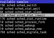
Vim help consists of 3.7 megabytes of text, half a million of words

$ wc neovim-0.3.4/runtime/doc/* | tail -n1
  90804  543942 3592651 total

Also, almost every plugin you install has its own help so these numbers are not final.

Vim help topics are comprehensive, detailed and cross-referenced. You may be overwhelmed at first because there is a lot of information here. But don’t be discouraged – it’s much much more efficient and useful to read and grasp comprehensive help topic than mindlessly searching for blog posts or StackOverflow. If you could only learn one thing from this post – please, learn to love the Vim help system.

Some tips that helped me.

• :h patt then TAB to find help on the subject starting with patt
• :h patt then Ctrl-D to find help on the subject containing patt
• Vim help system is full of cross-references – you can jump back and forward just like with code by using Ctrl-] and Ctrl-T.

Or even better – read the :help help which is help on help!

Let’s look at the example, if you type :h word-m Vim will open help on word motions:

==============================================================================
4. Word motions						*word-motions*

<S-Right>	or					*<S-Right>* *w*
w			[count] words forward.  |exclusive| motion.

<C-Right>	or					*<C-Right>* *W*
W			[count] WORDS forward.  |exclusive| motion.

...

Here you can see the header Word motions, its tag word-motions that is used as a subject for :h command.

Next, you see the help itself describing word motions.

Note that there are some words that have some funky symbols around them or shown in different colors. Anything that doesn’t look like the plain text is a help topic by itself – you can jump into it by Ctrl-]. So in this example, we could find what is [count] or what is |exclusive| motion. And that’s enough for efficient using of Vim help.

Here are the things that I’ve found in Vim help:

• I’ve configured statusline with the help of :h statusline. All the blog posts were just a waste of time.
• :h ins-completion describes comprehensive builtin completion system. Now, I’m using Ctrl-X Ctrl-F to complete filenames in the current directory (useful to insert links in Markdown files). Also, whole line completion with Ctrl-X Ctrl-L is useful for editing data files.
• :h window-moving taught me that you can move splits around, e.g. Ctrl-w H will move current window to the left (it will also convert vertical split to horizontal). Also, the whole :h windows.txt is amazing.

Finally, I recommend to everyone familiar with Vim to review :h quickref from time to time.

3. Use missed core features

After I’ve learned to use Vim help I started to discover things that I’ve missed but that was always there.

Remember to check the help for each thing in this list – I’ve conveniently supplied Vim help command and a link to online help.

Auto commands

:help autocmd

Auto commands allow you to tune Vim behavior based on filename or filetype. Basically, it executes Vim commands on events.

I use it to set correct filetype for some exotic files like this

autocmd BufRead,BufNewFile *.pp setfiletype ruby
autocmd BufRead,BufNewFile alert.rules setfiletype yaml

Or to tune settings for particular filetype like this

autocmd FileType yaml set tabstop=2 shiftwidth=2

Other editors required me to install full-blown extensions like Puppet extension or YAML extension but with Vim I keep things simple and lightweight.

Persistent undo

:help undo-persistence

This feature is so awesome yet none of the other editors have it.

It sounds simple – when you exit Vim your edit history is saved so you can open the file again 2 days later and undo the changes.

Edit history is an important part of your context so I think once you get used to it you couldn’t use any other editor without this feature.

To enable persistent undo I’ve done this:

set undodir=~/.vim/undodir
set undofile

Bliss!

Clipboard

:help 'clipboard'

This one is actually more of a hard fix than a feature.

Clipboard in Linux is a complicated story. All these buffers and selections don’t make things understandable. And Vim makes it even more complicated with its registers.

For years I had these mappings

" C-c and C-v - Copy/Paste to global clipboard
vmap <C-c> "+yi
imap <C-v> <esc>"+gpi

that makes Ctrl-c and Ctrl-v work.

But why use two-key combos when you can use a simple y and p for copying and pasting?

Turns out, you can make it work very nice by using this single setting:

set clipboard+=unnamed

It makes y and p copy and paste to the “global” buffer that is used by other apps like the browser.

Mappings

:help mapping

What I like the most about Vim is that its normal mode allows you to use all keys for a command while others require to use some key combo based on modifier (Ctrl-o, Ctrl-s).

When you can use any key for a command it’s natural to use a single key shortcuts, e.g. p to paste the text.

And what is even more awesome is that you can map a key or a sequence of keys at your own will.

Here are my most used mappings:

nnoremap ; :Buffers<CR>
nnoremap f :Files<CR>
nnoremap T :Tags<CR>
nnoremap t :BTags<CR>
nnoremap s :Ag<CR>

NOTE: these mappings override default Vim motions and actions because I don’t use them. It may be better for you to map it via leader key. Anyway, read the help on what these letters do by default and decide whether you want to override them.

These mappings invoke fzf command (more on this later) using a single key.

If I need to go to some function I just press t and got the list of tags of the current file. Not Ctrl-t, not Shift-t, just t. Combined with fzf fuzzy find it’s very powerful.

True colors in Vim

:help termguicolors

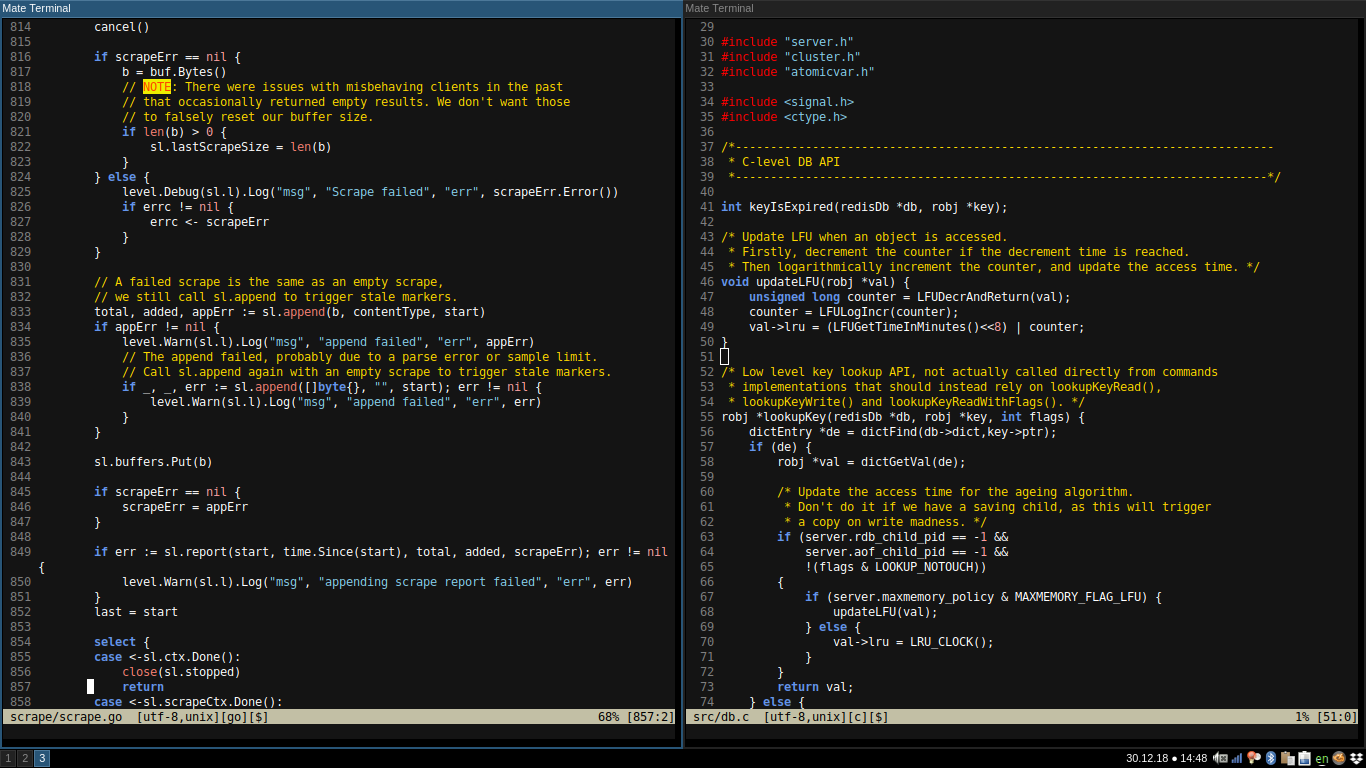
For years I’ve been using Vim in a terminal without knowing that I’ve been using 8-bit colorscheme. And it was actually ok because 256 colors is kinda enough.

It’s worth noting that I’m using my own colorscheme called tile. While tuning some of the colors I didn’t understand why I don’t see the difference and then I’ve read the help on syntax highlighting and realized that I want true colors in Vim.

Also, most of the colorschemes that you see in the wild, e.g. on https://vimcolors.com/ are presented in the 24-bit colors. So you’ll be disappointed when you don’t see the same colors when you install the colorscheme in your Vim.

Also also, your terminal is almost certainly capable of displaying in True Color so why limit yourself to the 256?

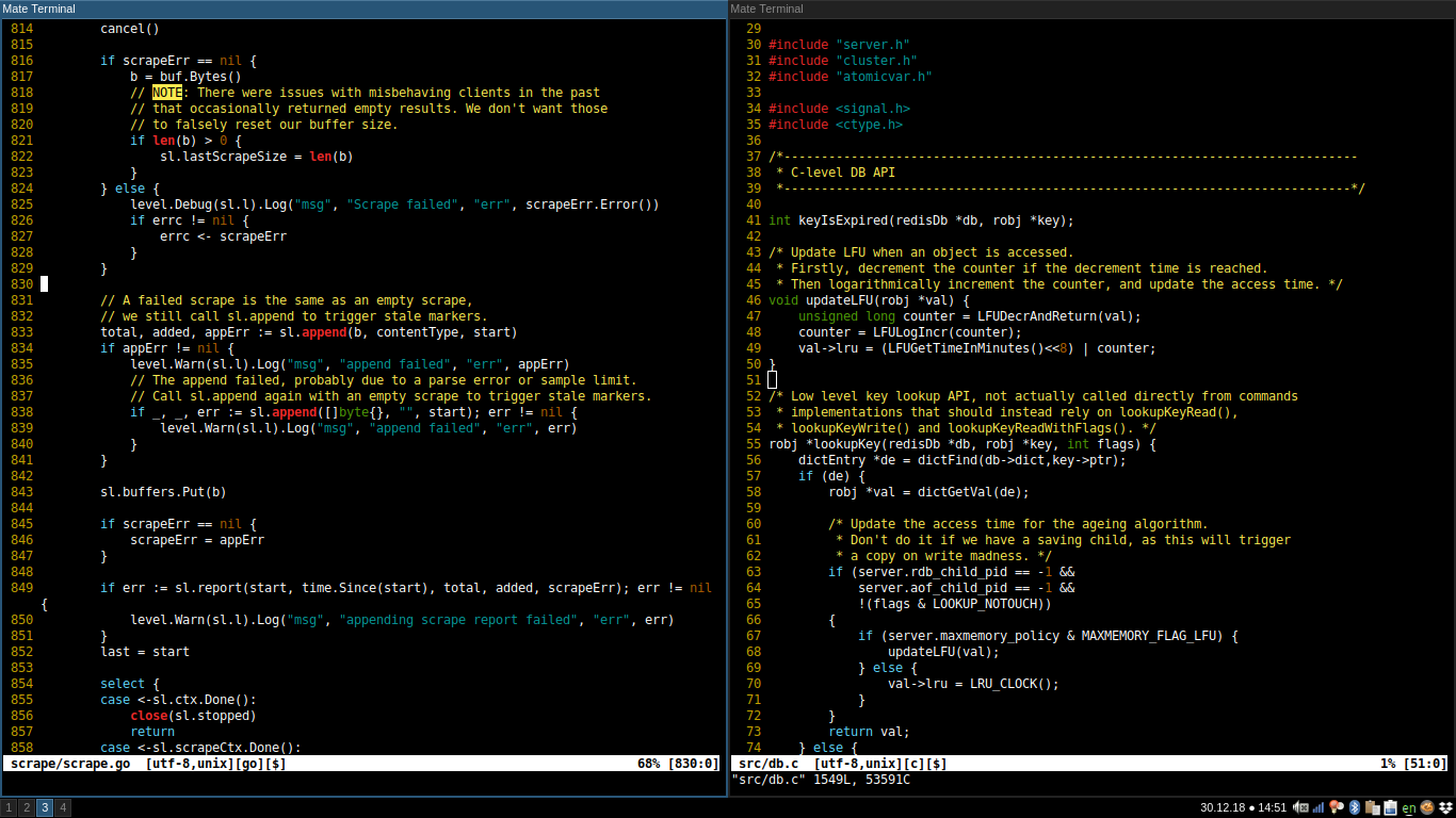
It’s all boils down to the simple set termguicolors in your vimrc. This options simply enable true color for Vim. Here is the difference with my colorscheme:

Search history

The last one is quick but so great that I even tweeted about it:

4. Tuning Vim to my workflow

All of the things above already boosted my productivity but Vim can do even better when you know what you want.

In my case, here was the list:

• Working with projects (sessions)
• Autocompletion
• Quick file find by fzf
• Quick search in files via ag (the_silver_searcher)
• Tag jumping using ctags index
• Find usages via cscope index
• Git integration (spoiler: no Fugitive)
• Linter integration
• Build integration
• Various niceties

So let’s dive in.

Working with projects

For me working with projects is about saving context – Open files, layout, cursor positions, settings, etc.

Vim has sessions (:help session) that does all that.

To save a session you have to :mksession! (or short :mks!) and then to load session start it with vim -S Session.vim. It may be enough for you but I found it kinda cumbersome to use as is.

First thing I’ve tried was to automate saving session. I’ve tried nice and simple obsession plugin that does just that. For the loading part, I’ve created bash alias alias vims='vim -S Session.vim'.

This was OK but a few things were annoying. The way I work is like this: I have multiple projects that are kept in separate directories as separate git repos. If I want to do something I cd into that dir, open the file, edit it or just view, and then do something else.

When I was opening a file with Vim inside a directory session wasn’t applied, so I had to manually :source it. After doing this for a week it was obvious that it’s not the way I wanted.

And then I’ve found an amazing vim-workspace plugin that does exactly what I need. It creates a session when you :ToggleWorkspace and keeps it updated. Then when you open any file in the workspace it automatically loads the session.

It also has very nice command :CloseHiddenBuffers that, well, closes hidden buffers. It’s very useful because during session lifetime you open files and Vim keeps them open. With this single command you can leave only the current buffer.

So I settled on the vim-workspace and found peace.

Autocompletion

Since the last time I’ve done Vim configuration, which was around 2008, a lot of things changes. But the most exploded sphere in Vim, from my point of view, was autocompletion support in Vim.

Vim gained sophisticated completion engine (:h ins-completion) with the omni-competion that gave birth to the whole load of plugins. YouCompleteMe, OmniCppComplete, neocomplcache/neocomplete/deoplete, AutoComplPop, clang_complete, …

It is complicated and I was exhausted while researching on this topic, so here is the shortest possible guide on completion plugins:

• YouCompleteMe – very powerful but huge plugin (>200 MB installed). Works as a client-server, requires a lot of utils.
• VimCompletesMe – a wrapper around Vim’s built-in completion hence super lightweight.
• Deoplete – current completion plugin by Shougo (previous were neocomplete and neocomplcache). Works as a client-server, much more lightweight than YouCompleteMe, can complete from a diverse set of sources.
• Other plugins are usually specific for concrete language.

My choice is deoplete because it’s fast, versatile, and not heavy. If you want to keep things native, then I’d recommend using VimCompletesMe. I’ve tried to use YouCompleteMe, had some troubles with installation, gave it 250 MB and it just showed me the function names without signatures and argument names. So I was disappointed and switched to deoplete that provides more info.

For the Deoplete I’ve added a few completion sources:

• Shougo/neco-syntax for generic syntax completion
• ujihisa/neco-look for dictionary completion – useful for writing blog posts.
• Shougo/deoplete-clangx for C/C++ completion
• deoplete-plugins/deoplete-go for Go completion
• deoplete-plugins/deoplete-jedi for Python completion

There is also tmux-complete that can complete from other tmux panes. Like view logs in one pane and Vim in the other pane can complete the values from it! It works but I don’t use tmux much.

There is also webcomplete completion source that completes from the currently open web page in Chrome. Alas, it works only on macos. There is an open discussion about adding support for Chrome on Linux.

Quick file find

The ability to quickly open file is crucial to my productivity. And I need to open a file by partial name. As an example, suppose I’m working in some ansible repo. I know that I have a template file for setting environment vars. I don’t remember exactly the full path but I know that it has env in it.

So I use fzf to sift through the list of file in the project that is generated by ag -l. Here is how it works live:

There are other plugins that do that like CtrlP but I use fzf for other things – list of buffers (open files), search, git commits, list of tags, history of search and history of command. Anything that should be sifted through is piped to the fzf because it does this job really well.

File find is launched with a single letter command f in the normal mode.

Quick search in files

Before this revamp I’ve used builtin / Vim command to search in the current buffer and :Ag to search in the files. I really like ag – it’s fast and very handy.

After I’ve embarked on the fzf I hooked Ag output to it and now it works even better:

File search is launched with a single letter command s in the normal mode.

Find usages

This was my long wished dream – when I stumble on some function I want to see its callers. Sounds simple but it’s a difficult task. The only thing that can do it and that is not tied to an IDE is cscope.

But cscope is a, how to say nice, weird thing. It requires you to build its own database by supplying a list of files and then provides tui interface to interact with. Its documentation doesn’t help much and it feels that nobody uses it.

This idiosyncratic cscope workflow was the main reason why I occasionally opted for other editors and IDEs. Just to see if they have “find usages” implemented well.

But this time I said to myself – you have to make it work. And here is what I did.

First, I started with automatically generating cscope database. I use vim-gutentags for this – it generates ctags index and cscope database on file save.

Then to integrate cscope I’ve tried different things:

• Tried to use CCTree but it builds its own cscope database and fails with some strange errors I don’t want to touch. So ditch it.
• Tried various cscope plugins – everything is just remapping of builtin cscope functions. No fzf support
• Finally settled on this thing based on https://gist.github.com/amitab/cd051f1ea23c588109c6cfcb7d1d5776

" cscope
function! Cscope(option, query)
  let color = '{ x = $1; $1 = ""; z = $3; $3 = ""; printf "\033[34m%s\033[0m:\033[31m%s\033[0m\011\033[37m%s\033[0m\n", x,z,$0; }'
  let opts = {
  \ 'source':  "cscope -dL" . a:option . " " . a:query . " | awk '" . color . "'",
  \ 'options': ['--ansi', '--prompt', '> ',
  \             '--multi', '--bind', 'alt-a:select-all,alt-d:deselect-all',
  \             '--color', 'fg:188,fg+:222,bg+:#3a3a3a,hl+:104'],
  \ 'down': '40%'
  \ }
  function! opts.sink(lines) 
    let data = split(a:lines)
    let file = split(data[0], ":")
    execute 'e ' . '+' . file[1] . ' ' . file[0]
  endfunction
  call fzf#run(opts)
endfunction

" Invoke command. 'g' is for call graph, kinda.
nnoremap <silent> <Leader>g :call Cscope('3', expand('<cword>'))<CR>

What it does is call cscope and feed its output to fzf. '3' is the field number in cscope TUI interface (yeah, you read it correct, :facepalm:) corresponding to Find functions calling this function.

This thing works – I pasted it to my vimrc and invoke it via <Leader>g but it needs to be packaged as a plugin. Maybe I’ll do this sometime.

Overall cscope feels like fucking dirt but we don’t have anything better.

Git integration

I’ve got used to console interface of git because it’s stable, independent of any editor and it provides all features of git because it’s the main interface. And I’m very comfortable with this way of working with git.

So my requirements for Git was pretty little – actually, I wanted to explore how this integration could help my workflow.

First, I’ve tried fugitive but quickly found that it was not for me. It was not suitable for my workflow. The main problem is that it messes my windows layout by opening its own buffers with git output:

• When I invoke :Gstatus I want to see the changes, so I invoke :Gdiff. It opens the diff in the closest window replacing buffer I was editing. That’s OK but when I’m done with the diff I want to close diff and return to the previous buffer. And this is where it gets complicated – diff is a 2 window, so I have to return with Ctrl-o to the previous buffer in one window and then kill the other buffer with :bd. This is really not convenient.
• :Glog just spits git log output in messages.
• :Gblame shows the standard git blame output and that’s OK. When I try to view commit from blame it opens it in the current window, again messing with my layout, and scrolls the commit to the diff of the chosen lines. This is not what I want, I want to view the commit message and other related changes. The scrolled part is what I already saw when I was doing blame.

So I’ve ditched it and settled on vim-gitgutter because it’s nice and doesn’t interfere with my workflow. This plugin shows line status in the gutter. And it provides a motion for next/previous hunk.

Then I’ve tried to use vimagit and it’s great! This is what I really want for Git integration – a convenient staging of changes and writing commit message. Vimagit gives me a buffer with unstaged and staged diffs and a commit message section and simple to use mappings. Really great!

Finally, I’ve found git-messenger that shows blame info (with history) in the floating window.

Build and linter integration

Similar to Git this wasn’t a hard requirement because I’m doing building and linting from the shell or automatically in CI. But, again, I wanted to explore what could be done here.

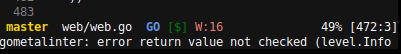
I setup Neomake as a linting engine. It has a pre-configured list of linters depending on filetype. I’ve configured it to run on only on buffer write (it can be launched at an interval, at reading, etc.) to avoid useless work. The count of warnings and errors of neomake run is shown in the in statusline (see screenshot below ). And the results of linting can be viewed in location list – :lopen, :lnext, :lprev.

Also, Neomake can invoke make program (:help makeprg) without blocking the UI so I’ve added this mapping and that’s it:

nnoremap <leader>m :Neomake!<cr>

The results of build are in the QuickFix list (:help quickfix).

Various niceties

ZoomWinTab

This plugin is a godsend for me. I use splits a lot and sometimes I want to temporary zoom the current window. With this plugin, I just do <Ctrl-w>z to toggle the zoom. This is similar to the tmux zoom feature.

Sensible

vim-sensible provides sensible defaults like enabling filetype, autoread, statusline. But most important for me was this line

set formatoptions+=j " Delete comment character when joining commented lines

Commentary

Commentary plugin adds actions to quickly comment line, selection or pretty much any motion.

Surround

Surround plugin allows me to easily add, change or delete “surroundings”. For example, I often use it to add quotes to the word with ysw" (I have a mapping for that) and change single quotes to double quotes with cs'".

Conclusion

So here I am, happily living with Vim for about 3 months now. I’ve intentionally waited from posting this to prove myself that my new setup is worth it. And, gosh, it is!

The main boost was getting comfortable with reading Vim help. Yes, I’m trying again to convince you about reading it because it makes you reason about what you do correctly.

And the key point is to tune Vim into your workflow, not the other way around.

Also, I’m tweaking things as I keep finding new ways to make my life in the editor more pleasant. The recent one was set hidden (:h hidden) to prevent nagging 'No write since last change' message when switching buffers.

There is no magic here in Vim when you put some conscientious effort and try to do things your way.

That’s it for now, till the next time!

Just in case you’ve never heard about it – Envoy is a proxy server that is most commonly used in a service mesh scenario but it’s also can be an edge proxy.

In this post, I will look only for edge proxy scenario because I’ve never maintained service mesh. Keep that use case in mind. Also, I will inevitably compare Envoy to nginx because that’s what I know and use.

What’s great about Envoy

The main reason why I wanted to try Envoy was its several compelling features:

• Observability
• Advanced load balancing policies
• Active checks
• Extensibility

Let’s unpack that list!

Observability

Observability is one of the most thorough features in Envoy. One of its design principles is to provide the transparency in network communication given how complex modern systems is built with all this microservices madness.

Out of the box it provides lots of metrics for various metrics system including Prometheus.

To get that kind of insight in nginx you have to buy nginx plus or use VTS module, thus compiling nginx on your own. Hopefully, my project nginx-vts-build will help – I’m building nginx with VTS module as a drop-in replacement for stock nginx with systemd service and basic configs. Think about it as nginx distro. Currently, it had only one release for Debian 9 but I’m open for suggestions. If you have a feature request, please let me know. But let’s get back to Envoy.

In addition to metrics, Envoy can be integrated with distributed tracing systems like Jaeger.

And finally, it can capture the traffic for further analysis with wireshark.

I’ve only looked at Prometheus metrics and they are quite nice!

Advanced load balancing

Load balancing in Envoy is very feature-rich. Not only it supports round-robin, weighted and random policies but also load balancing using consistent hashing algorithms like ketama and maglev. The point of the latter is fewer changes in traffic patterns in case of rebalancing in the upstream cluster.

Again, you can get the same advanced features in nginx but only if you pay for nginx plus.

Active checks

To check the health of the upstream endpoints Envoy will actively send the request and expect the valid answer so this endpoint will remain in the upstream cluster. This is a very nice feature that open source nginx lacks (but nginx plus has).

Extensibility

You can configure Envoy as a Redis proxy, DynamoDB filter, MongoDB filter, grpc proxy, MySQL filter, Thrift filter.

This is not a killer feature, imho, given that most of these protocols support is experimental but anyway it’s nice to have and shows that Envoy is extensible.

It also supports Lua scripting out of the box. For nginx you have to use OpenResty.

What’s not so great about Envoy

The features above alone make a very good reason to use Envoy. However, I found a few things that keep me from switching to Envoy from nginx:

• No caching
• No static content serving
• Lack of flexible configuration
• Docker-only packaging

No caching

Envoy doesn’t support caching of responses. This is a must-have feature for the edge proxy and nginx implements it really good.

No static content serving

While Envoy does networking really well, it doesn’t access filesystem apart from initial config file loading and runtime configuration handling. If you thought about serving static files like frontend things (js, html, css) then you’re out of luck - Envoy doesn’t support that. Nginx, again, does it very well.

Lack of flexible configuration

Envoy is configured via YAML and for me its configuration feels very explicit though I think it’s actually a good thing – explicit is better than implicit. But I feel that Envoy configuration is bounded by features specifically implemented in Envoy. Maybe it’s a lack of experience with Envoy and old habits but I feel that in nginx with maps, rewrite module (with if directive) and other nice modules I have a very flexible config system that allows me to implement anything. The cost of this flexibility is, of course, a good portion of complexity – nginx configuration requires some learning and practice but in my opinion it’s worth it.

Nevertheless, Envoy supports dynamic configuration, though it’s not like you can change some configuration part via REST call, it’s about the discovery of configuration settings – that’s what the whole XDS protocol is all about with its EDS, CDS, RDS and what-not-DS.

Citing docs:

Envoy discovers its various dynamic resources via the filesystem or by querying one or more management servers.

Emphasis is mine – I wanted to note that you have to provide a server that will respond to the Envoy discovery (XDS) requests.

However, there is no ready-made solution that implements Envoys’ XDS protocol. There was a rotor but the company behind it shut down so the project is mostly dead.

There is an Istio but it’s a monster I don’t want to touch right now. Also, if you’re on Kubernetes then there is a Heptio Contour, but not everybody needs and uses Kubernetes.

In the end, you could implement your own XDS service using go-control-plane stubs.

But that’s doesn’t seem to be used. What I saw most people do is using DNS for EDS and CDS. Especially, remembering that Consul has DNS interface, it seems that we can use Consul for dynamically providing the list of hosts to the Envoy. This isn’t big news because I can (and do) use Consul to provide the list of backends for nginx by using DNS name in proxy_pass and resolver directive.

Also, Consul Connect support Envoy for proxying requests but this is not about Envoy – this is about how awesome Consul is!

So this whole dynamic configuration thing of Envoy is really confusing and hard to follow because whenever you try to google it you’ll get bombarded with posts about Istio which is distracting.

Docker-only packaging

This is a minor thing but it just annoys me. Also, I don’t like that Docker images don’t have tags with versions. Maybe it’s intended so you always run the latest version but it seems very strange.

Conclusion on not-so-great parts

In the end, I’m not saying Envoy is bad in any way – from my point of view it just has a different focus on advanced proxying and out of process service mesh data plane. The edge proxy part is just a bonus that is suitable in some but not many situations.

What about mirroring

With that being said let’s see Envoy in practice and repeat mirroring experiments from my previous post.

Here are 2 minimal configs – one for nginx and the other Envoy. Both doing the same – simply proxying requests to some backend service.

# nginx proxy config

upstream backend {
    server backend.local:10000;
}

server {
    server_name proxy.local;
    listen 8000;

    location / {
        proxy_pass http://backend;
    }
}

# Envoy proxy config
static_resources:
  listeners:
  - name: listener_0
    address:
      socket_address:
        protocol: TCP
        address: 0.0.0.0
        port_value: 8001
    filter_chains:
    - filters:
      - name: envoy.http_connection_manager
        config:
          stat_prefix: ingress_http
          route_config:
            virtual_hosts:
            - name: local_service
              domains: ['*']
              routes:
              - match:
                  prefix: "/"
                route:
                  cluster: backend
          http_filters:
          - name: envoy.router
  clusters:
  - name: backend
    type: STATIC
    connect_timeout: 1s
    hosts:
      - socket_address:
          address: 127.0.0.1
          port_value: 10000

They perform identical:

$ # Load test nginx
$ hey -z 10s -q 1000 -c 1 -t 1 http://proxy.local:8000

Summary:
  Total:	10.0006 secs
  Slowest:	0.0229 secs
  Fastest:	0.0002 secs
  Average:	0.0004 secs
  Requests/sec:	996.7418
  
  Total data:	36881600 bytes
  Size/request:	3700 bytes

Response time histogram:
  0.000 [1]	|
  0.002 [9963]	|■■■■■■■■■■■■■■■■■■■■■■■■■■■■■■■■■■■■■■■■
  0.005 [3]	|
  0.007 [0]	|
  0.009 [0]	|
  0.012 [0]	|
  0.014 [0]	|
  0.016 [0]	|
  0.018 [0]	|
  0.021 [0]	|
  0.023 [1]	|

...

Status code distribution:
  [200]	9968 responses

$ # Load test Envoy
$ hey -z 10s -q 1000 -c 1 -t 1 http://proxy.local:8001

Summary:
  Total:	10.0006 secs
  Slowest:	0.0307 secs
  Fastest:	0.0003 secs
  Average:	0.0007 secs
  Requests/sec:	996.1445
  
  Total data:	36859400 bytes
  Size/request:	3700 bytes

Response time histogram:
  0.000 [1]	|
  0.003 [9960]	|■■■■■■■■■■■■■■■■■■■■■■■■■■■■■■■■■■■■■■■■
  0.006 [0]	|
  0.009 [0]	|
  0.012 [0]	|
  0.015 [0]	|
  0.019 [0]	|
  0.022 [0]	|
  0.025 [0]	|
  0.028 [0]	|
  0.031 [1]	|

...

Status code distribution:
  [200]	9962 responses

Anyway, let’s check the crucial part – mirroring to the backend with a delay. A quick reminder – nginx, in that case, will throttle original request thus affecting your production users.

Here is the mirroring config for Envoy:

# Envoy mirroring config
static_resources:
  listeners:
  - name: listener_0
    address:
      socket_address:
        protocol: TCP
        address: 0.0.0.0
        port_value: 8001
    filter_chains:
    - filters:
      - name: envoy.http_connection_manager
        config:
          stat_prefix: ingress_http
          route_config:
            virtual_hosts:
            - name: local_service
              domains: ['*']
              routes:
              - match:
                  prefix: "/"
                route:
                  cluster: backend
                  request_mirror_policy:
                    cluster: mirror
          http_filters:
          - name: envoy.router
  clusters:
  - name: backend
    type: STATIC
    connect_timeout: 1s
    hosts:
      - socket_address:
          address: 127.0.0.1
          port_value: 10000
  - name: mirror
    type: STATIC
    connect_timeout: 1s
    hosts:
      - socket_address:
          address: 127.0.0.1
          port_value: 20000

Basically, we’ve added request_mirror_policy to the main route and defined the cluster for mirroring. Let’s load test it!

$ hey -z 10s -q 1000 -c 1 -t 1 http://proxy.local:8001

Summary:
  Total:	10.0012 secs
  Slowest:	0.0046 secs
  Fastest:	0.0003 secs
  Average:	0.0008 secs
  Requests/sec:	997.6801
  
  Total data:	36918600 bytes
  Size/request:	3700 bytes

Response time histogram:
  0.000 [1]	|
  0.001 [2983]	|■■■■■■■■■■■■■■■■■
  0.001 [6916]	|■■■■■■■■■■■■■■■■■■■■■■■■■■■■■■■■■■■■■■■■
  0.002 [72]	|
  0.002 [2]	|
  0.002 [0]	|
  0.003 [0]	|
  0.003 [3]	|
  0.004 [0]	|
  0.004 [0]	|
  0.005 [1]	|

...

Status code distribution:
  [200]	9978 responses

Zero errors and amazing latency! This is a victory and it proves that Envoy’s mirroring is truly “fire and forget”!

Conclusion

Envoy’s networking is of exceptional quality – its mirroring is well thought, its load balancing is very advanced and I like the active health check feature.

I’m not convinced to use it in the edge proxy scenario because you might need features of a web server like caching, content serving and advanced configuration.

As for the service mesh – I’ll surely evaluate Envoy for that when the opportunity arises, so stay tuned – subscribe to the Atom feed and check my twitter @AlexDzyoba.

That’s it for now, till the next time!

• Pre-production testing by observing how your new system handle real production traffic
• Logging of requests for security analysis. This is what Wallarm tool do
• Copying requests for data science research
• etc.

I’ve used it for pre-production testing of the new rewritten system to see how well (if at all ;-) it can handle the production workload. There are some non-obvious problems and tips that I didn’t find when I started this journey and now I wanted to share it.

Basic setup

Let’s begin with a simple setup. Say, we have some backend that handles production workload and we put a proxy in front of it:

Here is the nginx config:

upstream backend {
    server backend.local:10000;
}

server {
    server_name proxy.local;
    listen 8000;

    location / {
        proxy_pass http://backend;
    }
}

There are 2 parts – backend and proxy. The proxy (nginx) is listening on port 8000 and just passing requests to the backend on port 10000. Nothing fancy, but let’s do a quick load test to see how it performs. I’m using hey tool because it’s simple and allows generating constant load instead of bombarding as hard as possible like many other tools do (wrk, apache benchmark, siege).

$ hey -z 10s -q 1000 -n 100000 -c 1 -t 1 http://proxy.local:8000

Summary:
  Total:	10.0016 secs
  Slowest:	0.0225 secs
  Fastest:	0.0003 secs
  Average:	0.0005 secs
  Requests/sec:	995.8393

  Total data:	6095520 bytes
  Size/request:	612 bytes

Response time histogram:
  0.000 [1]	|
  0.003 [9954]	|■■■■■■■■■■■■■■■■■■■■■■■■■■■■■■■■■■■■■■■■■■■
  0.005 [4]	|
  0.007 [0]	|
  0.009 [0]	|
  0.011 [0]	|
  0.014 [0]	|
  0.016 [0]	|
  0.018 [0]	|
  0.020 [0]	|
  0.022 [1]	|


Latency distribution:
  10% in 0.0003 secs
  25% in 0.0004 secs
  50% in 0.0005 secs
  75% in 0.0006 secs
  90% in 0.0007 secs
  95% in 0.0007 secs
  99% in 0.0009 secs

Details (average, fastest, slowest):
  DNS+dialup:	0.0000 secs, 0.0003 secs, 0.0225 secs
  DNS-lookup:	0.0000 secs, 0.0000 secs, 0.0008 secs
  req write:	0.0000 secs, 0.0000 secs, 0.0003 secs
  resp wait:	0.0004 secs, 0.0002 secs, 0.0198 secs
  resp read:	0.0001 secs, 0.0000 secs, 0.0012 secs

Status code distribution:
  [200]	9960 responses

Good, most of the requests are handled in less than a millisecond and there are no errors – that’s our baseline.

Basic mirroring

Now, let’s put another test backend and mirror traffic to it

The basic mirroring is configured like this:

upstream backend {
    server backend.local:10000;
}

upstream test_backend {
    server test.local:20000;
}

server {
    server_name proxy.local;
    listen 8000;

    location / {
        mirror /mirror;
        proxy_pass http://backend;
    }

    location = /mirror {
        internal;
        proxy_pass http://test_backend$request_uri;
    }

}

We add mirror directive to mirror requests to the internal location and define that internal location. In that internal location we can do whatever nginx allows us to do but for now we just simply proxy pass all requests.

Let’s load test it again to check how mirroring affects the performance:

$ hey -z 10s -q 1000 -n 100000 -c 1 -t 1 http://proxy.local:8000

Summary:
  Total:	10.0010 secs
  Slowest:	0.0042 secs
  Fastest:	0.0003 secs
  Average:	0.0005 secs
  Requests/sec:	997.3967

  Total data:	6104700 bytes
  Size/request:	612 bytes

Response time histogram:
  0.000 [1]	|
  0.001 [9132]	|■■■■■■■■■■■■■■■■■■■■■■■■■■■■■■■■■■■■■■■■
  0.001 [792]	|■■■
  0.001 [43]	|
  0.002 [3]	|
  0.002 [0]	|
  0.003 [2]	|
  0.003 [0]	|
  0.003 [0]	|
  0.004 [1]	|
  0.004 [1]	|


Latency distribution:
  10% in 0.0003 secs
  25% in 0.0004 secs
  50% in 0.0005 secs
  75% in 0.0006 secs
  90% in 0.0007 secs
  95% in 0.0008 secs
  99% in 0.0010 secs

Details (average, fastest, slowest):
  DNS+dialup:	0.0000 secs, 0.0003 secs, 0.0042 secs
  DNS-lookup:	0.0000 secs, 0.0000 secs, 0.0009 secs
  req write:	0.0000 secs, 0.0000 secs, 0.0002 secs
  resp wait:	0.0004 secs, 0.0002 secs, 0.0041 secs
  resp read:	0.0001 secs, 0.0000 secs, 0.0021 secs

Status code distribution:
  [200]	9975 responses

It’s pretty much the same – millisecond latency and no errors. And that’s good because it proves that mirroring itself doesn’t affect original requests.

Mirroring to buggy backend

That’s all nice and dandy but what if mirror backend has some bugs and sometimes replies with errors? What would happen to the original requests?

To test this I’ve made a trivial Go service that can inject errors randomly. Let’s launch it

$ mirror-backend -errors
2019/01/13 14:43:12 Listening on port 20000, delay is 0, error injecting is true

and see what load testing will show:

$ hey -z 10s -q 1000 -n 100000 -c 1 -t 1 http://proxy.local:8000

Summary:
  Total:	10.0008 secs
  Slowest:	0.0027 secs
  Fastest:	0.0003 secs
  Average:	0.0005 secs
  Requests/sec:	998.7205

  Total data:	6112656 bytes
  Size/request:	612 bytes

Response time histogram:
  0.000 [1]	|
  0.001 [7388]	|■■■■■■■■■■■■■■■■■■■■■■■■■■■■■■■■■■■■■■■■
  0.001 [2232]	|■■■■■■■■■■■■
  0.001 [324]	|■■
  0.001 [27]	|
  0.002 [6]	|
  0.002 [2]	|
  0.002 [3]	|
  0.002 [2]	|
  0.002 [0]	|
  0.003 [3]	|


Latency distribution:
  10% in 0.0003 secs
  25% in 0.0003 secs
  50% in 0.0004 secs
  75% in 0.0006 secs
  90% in 0.0007 secs
  95% in 0.0008 secs
  99% in 0.0009 secs

Details (average, fastest, slowest):
  DNS+dialup:	0.0000 secs, 0.0003 secs, 0.0027 secs
  DNS-lookup:	0.0000 secs, 0.0000 secs, 0.0008 secs
  req write:	0.0000 secs, 0.0000 secs, 0.0001 secs
  resp wait:	0.0004 secs, 0.0002 secs, 0.0026 secs
  resp read:	0.0001 secs, 0.0000 secs, 0.0006 secs

Status code distribution:
  [200]	9988 responses

Nothing changed at all! And that’s great because errors in the mirror backend don’t affect the main backend. nginx mirror module ignores responses to the mirror subrequests so this behavior is nice and intended.

Mirroring to a slow backend

But what if our mirror backend is not returning errors but just plain slow? How original requests will work? Let’s find out!

My mirror backend has an option to delay every request by configured amount of seconds. Here I’m launching it with a 1 second delay:

$ mirror-backend -delay 1
2019/01/13 14:50:39 Listening on port 20000, delay is 1, error injecting is false

So let’s see what load test show:

$ hey -z 10s -q 1000 -n 100000 -c 1 -t 1 http://proxy.local:8000

Summary:
  Total:	10.0290 secs
  Slowest:	0.0023 secs
  Fastest:	0.0018 secs
  Average:	0.0021 secs
  Requests/sec:	1.9942

  Total data:	6120 bytes
  Size/request:	612 bytes

Response time histogram:
  0.002 [1]	|■■■■■■■■■■
  0.002 [0]	|
  0.002 [1]	|■■■■■■■■■■
  0.002 [0]	|
  0.002 [0]	|
  0.002 [0]	|
  0.002 [1]	|■■■■■■■■■■
  0.002 [1]	|■■■■■■■■■■
  0.002 [0]	|
  0.002 [4]	|■■■■■■■■■■■■■■■■■■■■■■■■■■■■■■■■■■■■■■■■
  0.002 [2]	|■■■■■■■■■■■■■■■■■■■■


Latency distribution:
  10% in 0.0018 secs
  25% in 0.0021 secs
  50% in 0.0022 secs
  75% in 0.0023 secs
  90% in 0.0023 secs
  0% in 0.0000 secs
  0% in 0.0000 secs

Details (average, fastest, slowest):
  DNS+dialup:	0.0007 secs, 0.0018 secs, 0.0023 secs
  DNS-lookup:	0.0003 secs, 0.0002 secs, 0.0006 secs
  req write:	0.0001 secs, 0.0001 secs, 0.0002 secs
  resp wait:	0.0011 secs, 0.0007 secs, 0.0013 secs
  resp read:	0.0002 secs, 0.0001 secs, 0.0002 secs

Status code distribution:
  [200]	10 responses

Error distribution:
  [10]	Get http://proxy.local:8000: net/http: request canceled (Client.Timeout exceeded while awaiting headers)

What? 1.9 rps? Where is my 1000 rps? We’ve got errors? What’s happening?

Let me explain how mirroring in nginx works.

How mirroring in nginx works

When the request is coming to nginx and if mirroring is enabled, nginx will create a mirror subrequest and do what mirror location specifies – in our case, it will send it to the mirror backend.

But the thing is that subrequest is linked to the original request, so as far as I understand unless that mirror subrequest is not finished the original requests will throttle.

That’s why we get ~2 rps in the previous test – hey sent 10 requests, got responses, sent next 10 requests but they stalled because previous mirror subrequests were delayed and then timeout kicked in and errored the last 10 requests.

If we increase the timeout in hey to, say, 10 seconds we will receive no errors and 1 rps:

$ hey -z 10s -q 1000 -n 100000 -c 1 -t 10 http://proxy.local:8000

Summary:
  Total:	10.0197 secs
  Slowest:	1.0018 secs
  Fastest:	0.0020 secs
  Average:	0.9105 secs
  Requests/sec:	1.0978

  Total data:	6732 bytes
  Size/request:	612 bytes

Response time histogram:
  0.002 [1]	|■■■■
  0.102 [0]	|
  0.202 [0]	|
  0.302 [0]	|
  0.402 [0]	|
  0.502 [0]	|
  0.602 [0]	|
  0.702 [0]	|
  0.802 [0]	|
  0.902 [0]	|
  1.002 [10]	|■■■■■■■■■■■■■■■■■■■■■■■■■■■■■■■■■■■■■■■■


Latency distribution:
  10% in 1.0011 secs
  25% in 1.0012 secs
  50% in 1.0016 secs
  75% in 1.0016 secs
  90% in 1.0018 secs
  0% in 0.0000 secs
  0% in 0.0000 secs

Details (average, fastest, slowest):
  DNS+dialup:	0.0001 secs, 0.0020 secs, 1.0018 secs
  DNS-lookup:	0.0000 secs, 0.0000 secs, 0.0005 secs
  req write:	0.0001 secs, 0.0000 secs, 0.0002 secs
  resp wait:	0.9101 secs, 0.0008 secs, 1.0015 secs
  resp read:	0.0002 secs, 0.0001 secs, 0.0003 secs

Status code distribution:
  [200]	11 responses

So the point here is that if mirrored subrequests are slow then the original requests will be throttled. I don’t know how to fix this but I know the workaround – mirror only some part of the traffic. Let me show you how.

Mirroring part of the traffic

If you’re not sure that mirror backend can handle the original load you can mirror only some part of the traffic – for example, 10%.

mirror directive is not configurable and replicates all requests to the mirror location so it’s not obvious how to do this. The key point in achieving this is the internal mirror location. If you remember I’ve said that you can anything to mirrored requests in its location. So here is how I did this:

 1	upstream backend {
 2	    server backend.local:10000;
 3	}
 4	
 5	upstream test_backend {
 6	    server test.local:20000;
 7	}
 8	
 9	split_clients $remote_addr $mirror_backend {
10	    50% test_backend;
11	    *   "";
12	}
13	
14	server {
15	    server_name proxy.local;
16	    listen 8000;
17	
18	    access_log /var/log/nginx/proxy.log;
19	    error_log /var/log/nginx/proxy.error.log info;
20	
21	    location / {
22	        mirror /mirror;
23	        proxy_pass http://backend;
24	    }
25	
26	    location = /mirror {
27	        internal;
28	        if ($mirror_backend = "") {
29	            return 400;
30	        }
31	
32	        proxy_pass http://$mirror_backend$request_uri;
33	    }
34	
35	}
36	

First of all, in mirror location we proxy pass to the upstream that is taken from variable $mirror_backend (line 32). This variable is set in split_client block (lines 9-12) based on client remote address. What split_client does is it sets right variable value based on left variable distribution. In our case, we look at requests remote address ($remote_addr variable) and for 50% of remote addresses we set $mirror_backend to the test_backend, for other requests it’s set to empty string. Finally, the partial part is performed in mirror location – if $mirror_backend variable is empty we reject that mirror subrequest, otherwise we proxy_pass it. Remember that failure in mirror subrequests doesn’t affect original requests so it’s safe to drop request with error status.

The beauty of this solution is that you can split traffic for mirroring based on any variable or combination. If you want to really differentiate your users then remote address may not be the best split key – user may use many IPs or change them. In that case, you’re better off using some user-sticky key like API key. For mirroring 50% of traffic based on apikey query parameter we just change key in split_client:

split_clients $arg_apikey $mirror_backend {
    50% test_backend;
    *   "";
}

When we’ll query apikeys from 1 to 20 only half of it (11) will be mirrored. Here is the curl:

$ for i in {1..20};do curl -i "proxy.local:8000/?apikey=${i}" ;done

and here is the log of mirror backend:

...
2019/01/13 22:34:34 addr=127.0.0.1:47224 host=test_backend uri="/?apikey=1"
2019/01/13 22:34:34 addr=127.0.0.1:47230 host=test_backend uri="/?apikey=2"
2019/01/13 22:34:34 addr=127.0.0.1:47240 host=test_backend uri="/?apikey=4"
2019/01/13 22:34:34 addr=127.0.0.1:47246 host=test_backend uri="/?apikey=5"
2019/01/13 22:34:34 addr=127.0.0.1:47252 host=test_backend uri="/?apikey=6"
2019/01/13 22:34:34 addr=127.0.0.1:47262 host=test_backend uri="/?apikey=8"
2019/01/13 22:34:34 addr=127.0.0.1:47272 host=test_backend uri="/?apikey=10"
2019/01/13 22:34:34 addr=127.0.0.1:47278 host=test_backend uri="/?apikey=11"
2019/01/13 22:34:34 addr=127.0.0.1:47288 host=test_backend uri="/?apikey=13"
2019/01/13 22:34:34 addr=127.0.0.1:47298 host=test_backend uri="/?apikey=15"
2019/01/13 22:34:34 addr=127.0.0.1:47308 host=test_backend uri="/?apikey=17"
...

And the most awesome thing is that partitioning in split_client is consistent – requests with apikey=1 will always be mirrored.

Conclusion

So this was my experience with nginx mirror module so far. I’ve shown you how to simply mirror all of the traffic, how to mirror part of the traffic with the help of split_client module. I’ve also covered error handling and non-obvious problem when normal requests are throttled in case of slow mirror backend.

Hope you’ve enjoyed it! Subscribe to the Atom feed. I also post on twitter @AlexDzyoba.

That’s it for now, till the next time!

Imagine, you had an incident that happened at 11:45 your local time but your logs in ELK or Splunk are in UTC. So, what time was 11:45 in UTC?

$ tzconv utc 11:45
08:45

Boom! You got it!

You can add the third parameter to convert time from specific timezone, not from your local. For instance, your alert system sent you an email with a central European time and your server log timestamps are in Eastern time.

$ tzconv neyork 20:20 cet
14:20

Note, that I’ve mistyped New York and it still worked. That’s because locations are not matched exactly but fuzzy searched!

You can find more examples in the project README. Feel free to contribute, I’ve got a couple of things I would like to see implemented – check the issues page. The tool itself is written in Go and quite simple yet useful.

That’s it for now, till the next time!

Times were different back then and now we can have a really beefy server with the 10G network, 32 cores and 256 GiB RAM that can easily handle that amount of clients, so c10k is not much of a problem even with threaded I/O. But, anyway, I wanted to check how various solutions like threads and non-blocking async I/O will handle it, so I started to write some silly servers in my c10k repo and then I’ve stuck because I needed some tools to test my implementations.

Basically, I needed a c10k client. And I actually wrote a couple – one in Go and the other in C with libuv. I’m going to also write the one in Python 3 with asyncio.

While I was writing each client I’ve found 2 peculiarities – how to make it bad and how to make it slow.

How to make it bad

By making bad I mean making it really c10k – creating a lot of connections to the server thus saturation its resources.

Go client

I started with the client in Go and quickly stumbled upon the first roadblock. When I was making 10 concurrent HTTP request with simple "net/http" requests there were only 2 TCP connections

$ lsof -p $(pgrep go-client) -n -P
COMMAND     PID USER   FD      TYPE DEVICE SIZE/OFF    NODE NAME
go-client 11959  avd  cwd       DIR  253,0     4096 1183846 /home/avd/go/src/github.com/dzeban/c10k
go-client 11959  avd  rtd       DIR  253,0     4096       2 /
go-client 11959  avd  txt       REG  253,0  6240125 1186984 /home/avd/go/src/github.com/dzeban/c10k/go-client
go-client 11959  avd  mem       REG  253,0  2066456 3151328 /usr/lib64/libc-2.26.so
go-client 11959  avd  mem       REG  253,0   149360 3152802 /usr/lib64/libpthread-2.26.so
go-client 11959  avd  mem       REG  253,0   178464 3151302 /usr/lib64/ld-2.26.so
go-client 11959  avd    0u      CHR  136,0      0t0       3 /dev/pts/0
go-client 11959  avd    1u      CHR  136,0      0t0       3 /dev/pts/0
go-client 11959  avd    2u      CHR  136,0      0t0       3 /dev/pts/0
go-client 11959  avd    4u  a_inode   0,13        0   12735 [eventpoll]
go-client 11959  avd    8u     IPv4  68232      0t0     TCP 127.0.0.1:55224->127.0.0.1:80 (ESTABLISHED)
go-client 11959  avd   10u     IPv4  68235      0t0     TCP 127.0.0.1:55230->127.0.0.1:80 (ESTABLISHED)

The same with ss¹

$ ss -tnp dst 127.0.0.1:80
State  Recv-Q  Send-Q   Local Address:Port     Peer Address:Port
ESTAB  0       0         127.0.0.1:55224       127.0.0.1:80       users:(("go-client",pid=11959,fd=8))
ESTAB  0       0         127.0.0.1:55230       127.0.0.1:80       users:(("go-client",pid=11959,fd=10))

The reason for this is quite simple – HTTP 1.1 is using persistent connections with TCP keepalive for clients to avoid the overhead of TCP handshake on each HTTP request. Go’s "net/http" fully implements this logic – it multiplexes multiple requests over a handful of TCP connections. It can be tuned via Transport.

But I don’t need to tune it, I need to avoid it. And we can avoid it by explicitly creating TCP connection via net.Dial and then sending a single request over this connection. Here the function that does it and runs concurrently inside a dedicated goroutine.

func request(addr string, delay int, wg *sync.WaitGroup) {
	conn, err := net.Dial("tcp", addr)
	if err != nil {
		log.Fatal("dial error ", err)
	}

	req, err := http.NewRequest("GET", "/index.html", nil)
	if err != nil {
		log.Fatal("failed to create http request")
	}

	req.Host = "localhost"

	err = req.Write(conn)
	if err != nil {
		log.Fatal("failed to send http request")
	}

	_, err = bufio.NewReader(conn).ReadString('\n')
	if err != nil {
		log.Fatal("read error ", err)
	}

	wg.Done()
}

Let’s check it’s working

$ lsof -p $(pgrep go-client) -n -P
COMMAND     PID USER   FD      TYPE DEVICE SIZE/OFF    NODE NAME
go-client 12231  avd  cwd       DIR  253,0     4096 1183846 /home/avd/go/src/github.com/dzeban/c10k
go-client 12231  avd  rtd       DIR  253,0     4096       2 /
go-client 12231  avd  txt       REG  253,0  6167884 1186984 /home/avd/go/src/github.com/dzeban/c10k/go-client
go-client 12231  avd  mem       REG  253,0  2066456 3151328 /usr/lib64/libc-2.26.so
go-client 12231  avd  mem       REG  253,0   149360 3152802 /usr/lib64/libpthread-2.26.so
go-client 12231  avd  mem       REG  253,0   178464 3151302 /usr/lib64/ld-2.26.so
go-client 12231  avd    0u      CHR  136,0      0t0       3 /dev/pts/0
go-client 12231  avd    1u      CHR  136,0      0t0       3 /dev/pts/0
go-client 12231  avd    2u      CHR  136,0      0t0       3 /dev/pts/0
go-client 12231  avd    3u     IPv4  71768      0t0     TCP 127.0.0.1:55256->127.0.0.1:80 (ESTABLISHED)
go-client 12231  avd    4u  a_inode   0,13        0   12735 [eventpoll]
go-client 12231  avd    5u     IPv4  73753      0t0     TCP 127.0.0.1:55258->127.0.0.1:80 (ESTABLISHED)
go-client 12231  avd    6u     IPv4  71769      0t0     TCP 127.0.0.1:55266->127.0.0.1:80 (ESTABLISHED)
go-client 12231  avd    7u     IPv4  71770      0t0     TCP 127.0.0.1:55264->127.0.0.1:80 (ESTABLISHED)
go-client 12231  avd    8u     IPv4  73754      0t0     TCP 127.0.0.1:55260->127.0.0.1:80 (ESTABLISHED)
go-client 12231  avd    9u     IPv4  71771      0t0     TCP 127.0.0.1:55262->127.0.0.1:80 (ESTABLISHED)
go-client 12231  avd   10u     IPv4  71774      0t0     TCP 127.0.0.1:55268->127.0.0.1:80 (ESTABLISHED)
go-client 12231  avd   11u     IPv4  73755      0t0     TCP 127.0.0.1:55270->127.0.0.1:80 (ESTABLISHED)
go-client 12231  avd   12u     IPv4  71775      0t0     TCP 127.0.0.1:55272->127.0.0.1:80 (ESTABLISHED)
go-client 12231  avd   13u     IPv4  73758      0t0     TCP 127.0.0.1:55274->127.0.0.1:80 (ESTABLISHED)

$ ss -tnp dst 127.0.0.1:80
State  Recv-Q  Send-Q   Local Address:Port     Peer Address:Port
ESTAB  0       0         127.0.0.1:55260       127.0.0.1:80     users:(("go-client",pid=12231,fd=8))
ESTAB  0       0         127.0.0.1:55262       127.0.0.1:80     users:(("go-client",pid=12231,fd=9))
ESTAB  0       0         127.0.0.1:55270       127.0.0.1:80     users:(("go-client",pid=12231,fd=11))
ESTAB  0       0         127.0.0.1:55266       127.0.0.1:80     users:(("go-client",pid=12231,fd=6))
ESTAB  0       0         127.0.0.1:55256       127.0.0.1:80     users:(("go-client",pid=12231,fd=3))
ESTAB  0       0         127.0.0.1:55272       127.0.0.1:80     users:(("go-client",pid=12231,fd=12))
ESTAB  0       0         127.0.0.1:55258       127.0.0.1:80     users:(("go-client",pid=12231,fd=5))
ESTAB  0       0         127.0.0.1:55268       127.0.0.1:80     users:(("go-client",pid=12231,fd=10))
ESTAB  0       0         127.0.0.1:55264       127.0.0.1:80     users:(("go-client",pid=12231,fd=7))
ESTAB  0       0         127.0.0.1:55274       127.0.0.1:80     users:(("go-client",pid=12231,fd=13))

C client

I also decided to make a C client built on top of libuv for convenient event loop.

In my C client, there is no HTTP library so we’re making TCP connections from the start. It works well by creating a connection for each request so it doesn’t have the problem (more like feature :-) of the Go client. But when it finishes reading response it stucks and doesn’t return the control to the event loop until the very long timeout.

Here is the response reading callback that seems stuck:

static void on_read(uv_stream_t* stream, ssize_t nread, const uv_buf_t* buf)
{
    if (nread > 0) {
        printf("%s", buf->base);
    } else if (nread == UV_EOF) {
        log("close stream");
        uv_connect_t *conn = uv_handle_get_data((uv_handle_t *)stream);
        uv_close((uv_handle_t *)stream, free_close_cb);
        free(conn);
    } else {
        return_uv_err(nread);
    }

    free(buf->base);
}

It appears like we’re stuck here and wait for some (quite long) time until we finally got EOF.

This “quite long time” is actually HTTP keepalive timeout set in nginx and by default it’s 75 seconds.

We can control it on the client though with Connection and Keep-Alive HTTP headers which are part of HTTP 1.1.

And that’s the only sane solution because on the libuv side I had no way to close the convection – I don’t receive EOF because it is sent only when connection actually closed.

So what is happening is that my client creates a connection, send a request, nginx replies and then nginx is keeping connection because it waits for the subsequent requests. Tinkering with libuv showed me that and that’s why I love making things in C – you have to dig really deep and really understand how things work.

So to solve this hanging requests I’ve just set Connection: close header to enforce the new connection on each request from the same client and to disable HTTP keepalive. As an alternative, I could just insist on HTTP 1.0 where there is no keep-alive.

Now, that it’s creating lots of connections let’s make it keep those connections for a client-specified delay to appear a slow client.

How to make it slow

I needed to make it slow because I wanted my server to spend some time handling the requests while avoiding putting sleeps in the server code.

Initially, I thought to make reading on the client side slow, i.e. reading one byte at a time or delaying reading the server response. Interestingly, none of these solutions worked.

I tested my client with nginx by watching access log with the $request_time variable. Needless to say, all of my requests were served in 0.000 seconds. Whatever delay I’ve inserted, nginx seemed to ignore it.

I started to figure out why by tweaking various parts of the request-response pipeline like the number of connections, response size, etc.

Finally, I was able to see my delay only when nginx was serving really big file like 30 MB and that’s when it clicked.

The whole reason for this delay ignoring behavior were socket buffers. Socket buffers are, well, buffers for sockets, in other words, it’s the piece of memory where the Linux kernel buffers the network requests and responses for performance reason – to send data in big chunks over the network and to mitigate slow clients, and also for other things like TCP retransmission. Socket buffers are like page cache – all network I/O (with page cache it’s disk I/O) is made through it unless explicitly skipped.

So in my case, when nginx received a request, the response written by send/write syscall was merely stored in the socket buffer but from nginx point of view, it was done. Only when the response was large enough to not fit in the socket buffer, nginx would be blocked in syscall and wait until the client delay was elapsed, socket buffer was read and freed for the next portion of data.

You can check and tube the size of the socket buffers in /proc/sys/net/ipv4/tcp_rmem and /proc/sys/net/ipv4/tcp_wmem.

So after figuring this out, I’ve inserted delay after establishing the connection and before sending a request.

This way the server will keep around client connections (yay, c10k!) for a client-specified delay.

Recap

So in the end, I have a 2 c10k clients – one written in Go and the other written in C with libuv. The Python 3 client is on its way.

All of these clients connect to the HTTP server, waits for a specified delay and then sends GET request with Connection: close header.

This makes HTTP server keep a dedicated connection for each request and spend some time waiting to emulate I/O.

That’s how my c10k clients work.

1. Grokking data model and PromQL to get meaningful insights.
2. Configuring jmx-exporter.

In this post, I’ll share the JMX part because I don’t feel that I’ve fully understood the data model and PromQL. So let’s dive into that jmx-exporter thing.

What is jmx-exporter

jmx-exporter is a program that reads JMX data from JVM based applications (e.g. Java and Scala) and exposes it via HTTP in a simple text format that Prometheus understand and can scrape.

JMX is a common technology in Java world for exporting statistics of running application and also to control it (you can trigger GC with JMX, for example).

jmx-exporter is a Java application that uses JMX APIs to collect the app and JVM metrics. It is Java agent which means it is running inside the same JVM. This gives you a nice benefit of not exposing JMX remotely – jmx-exporter will just collect the metrics and exposes it over HTTP in read-only mode.

Installing jmx-exporter

Because it’s written in Java, jmx-exporter is distributed as a jar, so you just need to download it from maven and put it somewhere on your target host.

I have an Ansible role for this – https://github.com/alexdzyoba/ansible-jmx-exporter. Besides downloading the jar it’ll also put the configuration file for jmx-exporter.

This configuration file contains rules for rewriting JMX MBeans to the Prometheus exposition format metrics. Basically, it’s a collection of regexps to convert MBeans strings to Prometheus strings.

The example_configs directory in jmx-exporter sources contains examples for many popular Java apps including Kafka and Zookeeper.

Configuring Zookeeper with jmx-exporter

As I’ve said jmx-exporter runs inside other JVM as java agent to collect JMX metrics. To demonstrate how it all works, let’s run it within Zookeeper.

Zookeeper is a crucial part of many production systems including Hadoop, Kafka and Clickhouse, so you really want to monitor it. Despite the fact that you can do this with 4lw commands (mntr, stat, etc.) and that there are dedicated exporters I prefer to use JMX to avoid constant Zookeeper querying (they add noise to metrics because 4lw commands counted as normal Zookeeper requests).

To scrape Zookeeper JMX metrics with jmx-exporter you have to pass the following arguments to Zookeeper launch:

-javaagent:/opt/jmx-exporter/jmx-exporter.jar=7070:/etc/jmx-exporter/zookeeper.yml

If you use the Zookeeper that is distributed with Kafka (you shouldn’t) then pass it via EXTRA_ARGS:

$ export EXTRA_ARGS="-javaagent:/opt/jmx-exporter/jmx-exporter.jar=7070:/etc/jmx-exporter/zookeeper.yml"
$ /opt/kafka_2.11-0.10.1.0/bin/zookeeper-server-start.sh /opt/kafka_2.11-0.10.1.0/config/zookeeper.properties

If you use standalone Zookeeper distribution then add it as SERVER_JVMFLAGS to the zookeeper-env.sh:

# zookeeper-env.sh
SERVER_JVMFLAGS="-javaagent:/opt/jmx-exporter/jmx-exporter.jar=7070:/etc/jmx-exporter/zookeeper.yml"

Anyway, when you launch Zookeeper you should see the process listening on the specified port (7070 in my case) and responding to /metrics queries:

$ netstat -tlnp | grep 7070
tcp        0      0 0.0.0.0:7070            0.0.0.0:*               LISTEN      892/java

$ curl -s localhost:7070/metrics | head
# HELP jvm_threads_current Current thread count of a JVM
# TYPE jvm_threads_current gauge
jvm_threads_current 16.0
# HELP jvm_threads_daemon Daemon thread count of a JVM
# TYPE jvm_threads_daemon gauge
jvm_threads_daemon 12.0
# HELP jvm_threads_peak Peak thread count of a JVM
# TYPE jvm_threads_peak gauge
jvm_threads_peak 16.0
# HELP jvm_threads_started_total Started thread count of a JVM

Configuring Kafka with jmx-exporter

Kafka is a message broker written in Scala so it runs in JVM which in turn means that we can use jmx-exporter for its metrics.

To run jmx-exporter within Kafka, you should set KAFKA_OPTS environment variable like this:

$ export KAFKA_OPTS='-javaagent:/opt/jmx-exporter/jmx-exporter.jar=7071:/etc/jmx-exporter/kafka.yml'

Then launch the Kafka (I assume that Zookeeper is already launched as it’s required by Kafka):

$ /opt/kafka_2.11-0.10.1.0/bin/kafka-server-start.sh /opt/kafka_2.11-0.10.1.0/conf/server.properties

Check that jmx-exporter HTTP server is listening:

$ netstap -tlnp | grep 7071
tcp6       0      0 :::7071                 :::*                    LISTEN      19288/java

And scrape the metrics!

$ curl -s localhost:7071 | grep -i kafka | head
# HELP kafka_server_replicafetchermanager_minfetchrate Attribute exposed for management (kafka.server<type=ReplicaFetcherManager, name=MinFetchRate, clientId=Replica><>Value)
# TYPE kafka_server_replicafetchermanager_minfetchrate untyped
kafka_server_replicafetchermanager_minfetchrate{clientId="Replica",} 0.0
# HELP kafka_network_requestmetrics_totaltimems Attribute exposed for management (kafka.network<type=RequestMetrics, name=TotalTimeMs, request=OffsetFetch><>Count)
# TYPE kafka_network_requestmetrics_totaltimems untyped
kafka_network_requestmetrics_totaltimems{request="OffsetFetch",} 0.0
kafka_network_requestmetrics_totaltimems{request="JoinGroup",} 0.0
kafka_network_requestmetrics_totaltimems{request="DescribeGroups",} 0.0
kafka_network_requestmetrics_totaltimems{request="LeaveGroup",} 0.0
kafka_network_requestmetrics_totaltimems{request="GroupCoordinator",} 0.0

Here is how to run jmx-exporter java agent if you are running Kafka under systemd:

...
[Service]
Restart=on-failure
Environment=KAFKA_OPTS=-javaagent:/opt/jmx-exporter/jmx-exporter.jar=7071:/etc/jmx-exporter/kafka.yml
ExecStart=/opt/kafka/bin/kafka-server-start.sh /etc/kafka/server.properties
ExecStop=/opt/kafka/bin/kafka-server-stop.sh
TimeoutStopSec=600
User=kafka
...

Recap

With jmx-exporter you can scrape the metrics of running JVM applications. jmx-exporter runs as a Java agent (inside the target JVM) scrapes JMX metrics, rewrite it according to config rules and exposes it in Prometheus exposition format.

For a quick setup check my Ansible role for jmx-exporter alexdzyoba.jmx-exporter.

That’s all for now, stay tuned by subscribing to the RSS or follow me on Twitter @AlexDzyoba.

This post will cover tricky cases with cross-replicated cluster only because that’s what I use. If you have a plain flat topology with single Redis instances on the dedicated nodes you’ll be fine. But it’s not my case.

So let’s dive in.

Intro

First, let’s define some terms so we understand each other.

• Node – physical server or VM where you will run the Redis instance.
• Instance – Redis server process in a cluster mode.

Second, let me describe how my Redis cluster topology looks like and what is cross-replication.

Redis cluster is built from multiple Redis instances that are run in a cluster mode. Each instance is isolated because it serves a particular subset of keys in a master or slave role. The emphasis on the role is intentional – there is separate Redis instance for every shard master and every shard replica, e.g. if you have 3 shards with replication factor 3 (2 additional replicas) you have to run 9 Redis instances. This was my first naive attempt to create a cluster on 3 nodes:

$ redis-trib create --replicas 2 10.135.78.153:7000 10.135.78.196:7000 10.135.64.55:7000
>>> Creating cluster
*** ERROR: Invalid configuration for cluster creation.
*** Redis Cluster requires at least 3 master nodes.
*** This is not possible with 3 nodes and 2 replicas per node.
*** At least 9 nodes are required.

(redis-trib is an “official” tool to create a Redis cluster)

The important point here is that all of the Redis tools operate with Redis instances, not nodes, so it’s your responsibility to put the instances in the right redundant topology.

The motivation for cross replication

Redis cluster requires at least 3 nodes because to survive network partition it needs a masters majority (like in Sentinel). If you want 1 replica than add another 3 nodes and boom! now you have a 6 nodes cluster to operate.

It’s fine if you work in the cloud where you can just spin up a dozen of small nodes that cost you a little. Unfortunately, not everyone joined the cloud party and have to operate real metal nodes and server hardware usually starts with something like 32 GiB of RAM and 8 core CPU which is a real overkill for a Redis node.

So to save on hardware we can make a trick and run several instances on a single node (and probably colocate it with other services). But remember that in that case, you have to distribute masters among nodes manually and configure cross-replication.

Cross replication simply means that you don’t have dedicated nodes for replicas, you just replicate the data to the next node.

This way you save on the cluster size – you can make a Redis cluster with 2 replicas on 3 nodes instead of 9. So you have fewer things to operate and nodes are better utilized – instead of one single-threaded lightweight Redis process per 9 nodes now you’ll have 3 such processes on 3 nodes.

To create a cluster you have to run a redis-server with cluster-enabled yes parameter. With a cross-replicated cluster you run multiple Redis instances on a node, so you have to run it on separate ports. You can check these two manuals for details but the essential part are configs. This is the config file I’m using:

protected-mode no
port {{ redis_port }}
daemonize no
loglevel notice
logfile ""
cluster-enabled yes
cluster-config-file nodes-{{ redis_port }}.conf
cluster-node-timeout 5000
cluster-require-full-coverage no
cluster-slave-validity-factor 0

The redis_port variable takes 7000, 7001 and 7002 values for each shard. Launch 3 instances of Redis server with 7000, 7001 and 7002 on each of 3 nodes so you’ll have 9 instances total and let’s continue.

Building a cross-replicated cluster

The first surprise may hit you when you’ll build the cluster. If you invoke the redis-trib like this

$ redis-trib create --replicas 2 10.135.78.153:7000 10.135.78.196:7000 10.135.64.55:7000 10.135.78.153:7001 10.135.78.196:7001 10.135.64.55:7001 10.135.78.153:7002 10.135.78.196:7002 10.135.64.55:7002 

then it may put all your master instances on a single node. This is happening because, again, it assumes that each instance lives on the separate node.

So you have to distribute masters and slaves by hand. To do so, first, create a cluster from masters and then add slaves for each master.

# Create a cluster with masters
$ redis-trib create 10.135.78.153:7000 10.135.78.196:7001 10.135.64.55:7002
>>> Creating cluster
>>> Performing hash slots allocation on 3 nodes...
Using 3 masters:
10.135.78.153:7000
10.135.78.196:7001
10.135.64.55:7002
M: 763646767dd5492366c3c9f2978faa022833b7af 10.135.78.153:7000
slots:0-5460 (5461 slots) master
M: f63c210b13d68fa5dc97ca078af6d9c167f8c6ec 10.135.78.196:7001
slots:5461-10922 (5462 slots) master
M: 5f4bb09230ca016e7ffe2e6a4e5a32470175fb66 10.135.64.55:7002
slots:10923-16383 (5461 slots) master
Can I set the above configuration? (type 'yes' to accept): yes
>>> Nodes configuration updated
>>> Assign a different config epoch to each node
>>> Sending CLUSTER MEET messages to join the cluster
Waiting for the cluster to join.
>>> Performing Cluster Check (using node 10.135.78.153:7000)
M: 763646767dd5492366c3c9f2978faa022833b7af 10.135.78.153:7000
slots:0-5460 (5461 slots) master
0 additional replica(s)
M: 5f4bb09230ca016e7ffe2e6a4e5a32470175fb66 10.135.64.55:7002
slots:10923-16383 (5461 slots) master
0 additional replica(s)
M: f63c210b13d68fa5dc97ca078af6d9c167f8c6ec 10.135.78.196:7001
slots:5461-10922 (5462 slots) master
0 additional replica(s)
[OK] All nodes agree about slots configuration.
>>> Check for open slots...
>>> Check slots coverage...
[OK] All 16384 slots covered.

This is our cluster now:

127.0.0.1:7000> CLUSTER NODES                
763646767dd5492366c3c9f2978faa022833b7af 10.135.78.153:7000@17000 myself,master - 0 1524041299000 1 connected 0-5460
f63c210b13d68fa5dc97ca078af6d9c167f8c6ec 10.135.78.196:7001@17001 master - 0 1524041299426 2 connected 5461-10922
5f4bb09230ca016e7ffe2e6a4e5a32470175fb66 10.135.64.55:7002@17002 master - 0 1524041298408 3 connected 10923-16383

Now add 2 replicas for each master:

$ redis-trib add-node --slave --master-id 763646767dd5492366c3c9f2978faa022833b7af 10.135.78.196:7000 10.135.78.153:7000
$ redis-trib add-node --slave --master-id 763646767dd5492366c3c9f2978faa022833b7af 10.135.64.55:7000 10.135.78.153:7000

$ redis-trib add-node --slave --master-id f63c210b13d68fa5dc97ca078af6d9c167f8c6ec 10.135.78.153:7001 10.135.78.153:7000
$ redis-trib add-node --slave --master-id f63c210b13d68fa5dc97ca078af6d9c167f8c6ec 10.135.64.55:7001 10.135.78.153:7000

$ redis-trib add-node --slave --master-id 5f4bb09230ca016e7ffe2e6a4e5a32470175fb66 10.135.78.153:7002 10.135.78.153:7000
$ redis-trib add-node --slave --master-id 5f4bb09230ca016e7ffe2e6a4e5a32470175fb66 10.135.78.196:7002 10.135.78.153:7000

Now, this is our brand new cross replicated cluster with 2 replicas:

$ redis-cli -c -p 7000 cluster nodes
763646767dd5492366c3c9f2978faa022833b7af 10.135.78.153:7000@17000 myself,master - 0 1524041947000 1 connected 0-5460
216a5ea51af1faed7fa42b0c153c91855f769321 10.135.78.196:7000@17000 slave 763646767dd5492366c3c9f2978faa022833b7af 0 1524041948515 1 connected
0441f7534aed16123bb3476124506251dab80747 10.135.64.55:7000@17000 slave 763646767dd5492366c3c9f2978faa022833b7af 0 1524041947094 1 connected
f63c210b13d68fa5dc97ca078af6d9c167f8c6ec 10.135.78.196:7001@17001 master - 0 1524043602115 2 connected 5461-10922
f90c932d5cf435c75697dc984b0cbb94c130f115 10.135.78.153:7001@17001 slave f63c210b13d68fa5dc97ca078af6d9c167f8c6ec 0 1524043601595 2 connected
00eb2402fc1868763a393ae2c9843c47cd7d49da 10.135.64.55:7001@17001 slave f63c210b13d68fa5dc97ca078af6d9c167f8c6ec 0 1524043600057 2 connected
5f4bb09230ca016e7ffe2e6a4e5a32470175fb66 10.135.64.55:7002@17002 master - 0 1524041948515 3 connected 10923-16383
af75fc17e552279e5939bfe2df68075b3b6f9b29 10.135.78.153:7002@17002 slave 5f4bb09230ca016e7ffe2e6a4e5a32470175fb66 0 1524041948000 3 connected
19b8c9f7ac472ecfedd109e6bb7a4b932905c4fd 10.135.78.196:7002@17002 slave 5f4bb09230ca016e7ffe2e6a4e5a32470175fb66 0 1524041947094 3 connected

Failover of a cluster node

If we fail (with DEBUG SEGFAULT command) our third node (10.135.64.55) cluster will continue to work:

127.0.0.1:7000> CLUSTER NODES
763646767dd5492366c3c9f2978faa022833b7af 10.135.78.153:7000@17000 myself,master - 0 1524043923000 1 connected 0-5460
216a5ea51af1faed7fa42b0c153c91855f769321 10.135.78.196:7000@17000 slave 763646767dd5492366c3c9f2978faa022833b7af 0 1524043924569 1 connected
0441f7534aed16123bb3476124506251dab80747 10.135.64.55:7000@17000 slave,fail 763646767dd5492366c3c9f2978faa022833b7af 1524043857000 1524043856593 1 disconnected
f63c210b13d68fa5dc97ca078af6d9c167f8c6ec 10.135.78.196:7001@17001 master - 0 1524043924874 2 connected 5461-10922
f90c932d5cf435c75697dc984b0cbb94c130f115 10.135.78.153:7001@17001 slave f63c210b13d68fa5dc97ca078af6d9c167f8c6ec 0 1524043924000 2 connected
00eb2402fc1868763a393ae2c9843c47cd7d49da 10.135.64.55:7001@17001 slave,fail f63c210b13d68fa5dc97ca078af6d9c167f8c6ec 1524043862669 1524043862000 2 disconnected
5f4bb09230ca016e7ffe2e6a4e5a32470175fb66 10.135.64.55:7002@17002 master,fail - 1524043864490 1524043862567 3 disconnected
af75fc17e552279e5939bfe2df68075b3b6f9b29 10.135.78.153:7002@17002 slave 19b8c9f7ac472ecfedd109e6bb7a4b932905c4fd 0 1524043924568 4 connected
19b8c9f7ac472ecfedd109e6bb7a4b932905c4fd 10.135.78.196:7002@17002 master - 0 1524043924000 4 connected 10923-16383

We can see that replica on 10.135.78.196:7002 took over the slot range 10923-16383 and now it’s master

127.0.0.1:7000> set a 2
-> Redirected to slot [15495] located at 10.135.78.196:7002
OK

Should we restore Redis instances on the third node cluster will restore

127.0.0.1:7000> CLUSTER nodes
763646767dd5492366c3c9f2978faa022833b7af 10.135.78.153:7000@17000 myself,master - 0 1524044130000 1 connected 0-5460
216a5ea51af1faed7fa42b0c153c91855f769321 10.135.78.196:7000@17000 slave 763646767dd5492366c3c9f2978faa022833b7af 0 1524044131572 1 connected
0441f7534aed16123bb3476124506251dab80747 10.135.64.55:7000@17000 slave 763646767dd5492366c3c9f2978faa022833b7af 0 1524044131367 1 connected
f63c210b13d68fa5dc97ca078af6d9c167f8c6ec 10.135.78.196:7001@17001 master - 0 1524044130334 2 connected 5461-10922
f90c932d5cf435c75697dc984b0cbb94c130f115 10.135.78.153:7001@17001 slave f63c210b13d68fa5dc97ca078af6d9c167f8c6ec 0 1524044131876 2 connected
00eb2402fc1868763a393ae2c9843c47cd7d49da 10.135.64.55:7001@17001 slave f63c210b13d68fa5dc97ca078af6d9c167f8c6ec 0 1524044131877 2 connected
19b8c9f7ac472ecfedd109e6bb7a4b932905c4fd 10.135.78.196:7002@17002 master - 0 1524044131572 4 connected 10923-16383
af75fc17e552279e5939bfe2df68075b3b6f9b29 10.135.78.153:7002@17002 slave 19b8c9f7ac472ecfedd109e6bb7a4b932905c4fd 0 1524044131000 4 connected
5f4bb09230ca016e7ffe2e6a4e5a32470175fb66 10.135.64.55:7002@17002 slave 19b8c9f7ac472ecfedd109e6bb7a4b932905c4fd 0 1524044131572 4 connected

However, master was not restored back on original node, it’s still on the second node (10.135.78.196). After reboot the third node contains only slave instances

$ redis-cli -c -p 7000 cluster nodes | grep 10.135.64.55
0441f7534aed16123bb3476124506251dab80747 10.135.64.55:7000@17000 slave 763646767dd5492366c3c9f2978faa022833b7af 0 1524044294347 1 connected
00eb2402fc1868763a393ae2c9843c47cd7d49da 10.135.64.55:7001@17001 slave f63c210b13d68fa5dc97ca078af6d9c167f8c6ec 0 1524044293138 2 connected
5f4bb09230ca016e7ffe2e6a4e5a32470175fb66 10.135.64.55:7002@17002 slave 19b8c9f7ac472ecfedd109e6bb7a4b932905c4fd 0 1524044294553 4 connected

and the second node serve 2 master instances.

$ redis-cli -c -p 7000 cluster nodes | grep 10.135.78.196
216a5ea51af1faed7fa42b0c153c91855f769321 10.135.78.196:7000@17000 slave 763646767dd5492366c3c9f2978faa022833b7af 0 1524044345000 1 connected
f63c210b13d68fa5dc97ca078af6d9c167f8c6ec 10.135.78.196:7001@17001 master - 0 1524044345000 2 connected 5461-10922
19b8c9f7ac472ecfedd109e6bb7a4b932905c4fd 10.135.78.196:7002@17002 master - 0 1524044345000 4 connected 10923-16383

Now, what is interesting is that if the second node will fail in this state we’ll lose 2 out of 3 masters and we’ll lose the whole cluster because there is no masters quorum.

$ redis-cli -c -p 7000 cluster nodes
763646767dd5492366c3c9f2978faa022833b7af 10.135.78.153:7000@17000 myself,master - 0 1524046655000 1 connected 0-5460
216a5ea51af1faed7fa42b0c153c91855f769321 10.135.78.196:7000@17000 slave,fail 763646767dd5492366c3c9f2978faa022833b7af 1524046544940 1524046544000 1 disconnected
0441f7534aed16123bb3476124506251dab80747 10.135.64.55:7000@17000 slave 763646767dd5492366c3c9f2978faa022833b7af 0 1524046654010 1 connected
f63c210b13d68fa5dc97ca078af6d9c167f8c6ec 10.135.78.196:7001@17001 master,fail? - 1524046602511 1524046601582 2 disconnected 5461-10922
f90c932d5cf435c75697dc984b0cbb94c130f115 10.135.78.153:7001@17001 slave f63c210b13d68fa5dc97ca078af6d9c167f8c6ec 0 1524046655039 2 connected
00eb2402fc1868763a393ae2c9843c47cd7d49da 10.135.64.55:7001@17001 slave f63c210b13d68fa5dc97ca078af6d9c167f8c6ec 0 1524046656075 2 connected
19b8c9f7ac472ecfedd109e6bb7a4b932905c4fd 10.135.78.196:7002@17002 master,fail? - 1524046605581 1524046603746 4 disconnected 10923-16383
af75fc17e552279e5939bfe2df68075b3b6f9b29 10.135.78.153:7002@17002 slave 19b8c9f7ac472ecfedd109e6bb7a4b932905c4fd 0 1524046654623 4 connected
5f4bb09230ca016e7ffe2e6a4e5a32470175fb66 10.135.64.55:7002@17002 slave 19b8c9f7ac472ecfedd109e6bb7a4b932905c4fd 0 1524046654515 4 connected

Let me reiterate that – with cross replicated cluster you may lose the whole cluster after 2 consequent reboots of the single nodes. This is the reason why you’re better off with a dedicated node for each Redis instance, otherwise, with cross replication, we should really watch for masters distribution.

To avoid the situation above we should manually failover one of the slaves on the third node to become a master.

To do this we should connect to the 10.135.64.55:7002 which is replica now and then issue CLUSTER FAILOVER command:

127.0.0.1:7002> CLUSTER FAILOVER
OK

127.0.0.1:7002> CLUSTER NODES
763646767dd5492366c3c9f2978faa022833b7af 10.135.78.153:7000@17000 master - 0 1524047703000 1 connected 0-5460
216a5ea51af1faed7fa42b0c153c91855f769321 10.135.78.196:7000@17000 slave 763646767dd5492366c3c9f2978faa022833b7af 0 1524047703512 1 connected
0441f7534aed16123bb3476124506251dab80747 10.135.64.55:7000@17000 slave 763646767dd5492366c3c9f2978faa022833b7af 0 1524047703512 1 connected
f63c210b13d68fa5dc97ca078af6d9c167f8c6ec 10.135.78.196:7001@17001 master - 0 1524047703000 2 connected 5461-10922
f90c932d5cf435c75697dc984b0cbb94c130f115 10.135.78.153:7001@17001 slave f63c210b13d68fa5dc97ca078af6d9c167f8c6ec 0 1524047703000 2 connected
00eb2402fc1868763a393ae2c9843c47cd7d49da 10.135.64.55:7001@17001 slave f63c210b13d68fa5dc97ca078af6d9c167f8c6ec 0 1524047703110 2 connected
5f4bb09230ca016e7ffe2e6a4e5a32470175fb66 10.135.64.55:7002@17002 myself,master - 0 1524047703000 5 connected 10923-16383
af75fc17e552279e5939bfe2df68075b3b6f9b29 10.135.78.153:7002@17002 slave 5f4bb09230ca016e7ffe2e6a4e5a32470175fb66 0 1524047702510 5 connected
19b8c9f7ac472ecfedd109e6bb7a4b932905c4fd 10.135.78.196:7002@17002 slave 5f4bb09230ca016e7ffe2e6a4e5a32470175fb66 0 1524047702009 5 connected

Replacing a failed node

Now, suppose we’ve lost our third node completely and want to replace it with a completely new node.

$ redis-cli -c -p 7000 cluster nodes
763646767dd5492366c3c9f2978faa022833b7af 10.135.78.153:7000@17000 myself,master - 0 1524047906000 1 connected 0-5460
216a5ea51af1faed7fa42b0c153c91855f769321 10.135.78.196:7000@17000 slave 763646767dd5492366c3c9f2978faa022833b7af 0 1524047906811 1 connected
0441f7534aed16123bb3476124506251dab80747 10.135.64.55:7000@17000 slave,fail 763646767dd5492366c3c9f2978faa022833b7af 1524047871538 1524047869000 1 connected
f90c932d5cf435c75697dc984b0cbb94c130f115 10.135.78.153:7001@17001 slave f63c210b13d68fa5dc97ca078af6d9c167f8c6ec 0 1524047908000 2 connected
f63c210b13d68fa5dc97ca078af6d9c167f8c6ec 10.135.78.196:7001@17001 master - 0 1524047907318 2 connected 5461-10922
00eb2402fc1868763a393ae2c9843c47cd7d49da 10.135.64.55:7001@17001 slave,fail f63c210b13d68fa5dc97ca078af6d9c167f8c6ec 1524047872042 1524047869515 2 connected
19b8c9f7ac472ecfedd109e6bb7a4b932905c4fd 10.135.78.196:7002@17002 master - 0 1524047907000 6 connected 10923-16383
af75fc17e552279e5939bfe2df68075b3b6f9b29 10.135.78.153:7002@17002 slave 19b8c9f7ac472ecfedd109e6bb7a4b932905c4fd 0 1524047908336 6 connected
5f4bb09230ca016e7ffe2e6a4e5a32470175fb66 10.135.64.55:7002@17002 master,fail - 1524047871840 1524047869314 5 connected

First, we have to forget the lost node by issuing CLUSTER FORGET <node-id> on every single node of the cluster (even slaves).

for id in 0441f7534aed16123bb3476124506251dab80747 00eb2402fc1868763a393ae2c9843c47cd7d49da 5f4bb09230ca016e7ffe2e6a4e5a32470175fb66; do 
    for port in 7000 7001 7002; do 
        redis-cli -c -p ${port} CLUSTER FORGET ${id}
    done
done

Check that we’ve forgotten the failed node:

$ redis-cli -c -p 7000 cluster nodes
763646767dd5492366c3c9f2978faa022833b7af 10.135.78.153:7000@17000 myself,master - 0 1524048240000 1 connected 0-5460
216a5ea51af1faed7fa42b0c153c91855f769321 10.135.78.196:7000@17000 slave 763646767dd5492366c3c9f2978faa022833b7af 0 1524048241342 1 connected
f63c210b13d68fa5dc97ca078af6d9c167f8c6ec 10.135.78.196:7001@17001 master - 0 1524048240332 2 connected 5461-10922
f90c932d5cf435c75697dc984b0cbb94c130f115 10.135.78.153:7001@17001 slave f63c210b13d68fa5dc97ca078af6d9c167f8c6ec 0 1524048240000 2 connected
19b8c9f7ac472ecfedd109e6bb7a4b932905c4fd 10.135.78.196:7002@17002 master - 0 1524048241000 6 connected 10923-16383
af75fc17e552279e5939bfe2df68075b3b6f9b29 10.135.78.153:7002@17002 slave 19b8c9f7ac472ecfedd109e6bb7a4b932905c4fd 0 1524048241845 6 connected

Now spin up a new node, install redis on it and launch 3 new instances with our cluster configuration.

These 3 new nodes doesn’t know anything about the cluster:

[root@redis-replaced ~]# redis-cli -c -p 7000 cluster nodes
9a9c19e24e04df35ad54a8aff750475e707c8367 :7000@17000 myself,master - 0 0 0 connected
[root@redis-replaced ~]# redis-cli -c -p 7001 cluster nodes
3a35ebbb6160232d36984e7a5b97d430077e7eb0 :7001@17001 myself,master - 0 0 0 connected
[root@redis-replaced ~]# redis-cli -c -p 7002 cluster nodes
df701f8b24ae3c68ca6f9e1015d7362edccbb0ab :7002@17002 myself,master - 0 0 0 connected

so we have to add these Redis instances to the cluster:

$ redis-trib add-node --slave --master-id 763646767dd5492366c3c9f2978faa022833b7af 10.135.82.90:7000 10.135.78.153:7000
$ redis-trib add-node --slave --master-id f63c210b13d68fa5dc97ca078af6d9c167f8c6ec 10.135.82.90:7001 10.135.78.153:7000
$ redis-trib add-node --slave --master-id 19b8c9f7ac472ecfedd109e6bb7a4b932905c4fd 10.135.82.90:7002 10.135.78.153:7000

Now we should failover for the third shard:

[root@redis-replaced ~]# redis-cli -c -p 7002 cluster failover
OK

Aaaand, it’s done!

$ redis-cli -c -p 7000 cluster nodes
763646767dd5492366c3c9f2978faa022833b7af 10.135.78.153:7000@17000 myself,master - 0 1524049388000 1 connected 0-5460
f90c932d5cf435c75697dc984b0cbb94c130f115 10.135.78.153:7001@17001 slave f63c210b13d68fa5dc97ca078af6d9c167f8c6ec 0 1524049389000 2 connected
af75fc17e552279e5939bfe2df68075b3b6f9b29 10.135.78.153:7002@17002 slave df701f8b24ae3c68ca6f9e1015d7362edccbb0ab 0 1524049388000 7 connected
216a5ea51af1faed7fa42b0c153c91855f769321 10.135.78.196:7000@17000 slave 763646767dd5492366c3c9f2978faa022833b7af 0 1524049389579 1 connected
f63c210b13d68fa5dc97ca078af6d9c167f8c6ec 10.135.78.196:7001@17001 master - 0 1524049389579 2 connected 5461-10922
19b8c9f7ac472ecfedd109e6bb7a4b932905c4fd 10.135.78.196:7002@17002 slave df701f8b24ae3c68ca6f9e1015d7362edccbb0ab 0 1524049388565 7 connected
9a9c19e24e04df35ad54a8aff750475e707c8367 10.135.82.90:7000@17000 slave 763646767dd5492366c3c9f2978faa022833b7af 0 1524049389880 1 connected
3a35ebbb6160232d36984e7a5b97d430077e7eb0 10.135.82.90:7001@17001 slave f63c210b13d68fa5dc97ca078af6d9c167f8c6ec 0 1524049389579 2 connected
df701f8b24ae3c68ca6f9e1015d7362edccbb0ab 10.135.82.90:7002@17002 master - 0 1524049389579 7 connected 10923-16383

Recap

If you have to deal with bare metal servers, want a highly available Redis cluster and effectively utilize your hardware you have a good option of building cross replicated topology of Redis cluster.

This will work great but there are 2 caveats:

1. Cluster building is a manual process because you have to put masters on separate nodes.
2. You have to monitor your masters’ distribution to avoid cluster failure after a single node failure.

I’m going to describe high availability in terms of node failure and not persistence.

Redis high availability options

Standalone Redis, which is a good old redis-server you launch after installation, is easy to setup and use, but it’s not resilient to the failure of a node it’s running on. It doesn’t matter whether you use RDB or AOF as long as a node is unavailable you are in a trouble.

Over the years, Redis community came up with a few high availability options – most of them are built in Redis itself, though there are some others that are 3rd party tools. Let’s dive into it.

Simple Redis replication

Redis has a replication support since, like, forever and it works great – just put the slaveof <addr> <port> in your config file and the instance will start receiving the stream of the data from the master.

You can configure multiple slaves for the master, you can configure slave for a slave, you can enable slave-only persistence, you can make replication synchronous (it’s async by default) – the list of what you can do with Redis seems like bounded only by your imagination. Just read the docs for replication – it’s really great.

Pros:

• Quick and simple to setup
• Could be automated via configuration management tools
• Continue to work as long as a single master instance is available - it can survive failures of all of the slave instances.

Cons:

• Writes must go to the master
• Slaves may serve reads but because replication is asynchronous you may get stale reads
• It doesn’t shard data, so master and slaves will have unbalanced utilization
• In case of master failure, you have to elect the new master manually

The last thing is, IMHO, a major downside and that’s where the Redis Sentinel helps.

Redis replication with Sentinel

Nobody wants to wake up in the middle of the night, just to issue the SLAVEOF NO ONE to elect new master – it’s pretty silly and should be automated, right? Right. That’s why Redis Sentinel exists.

Redis Sentinel is the tool that monitors Redis masters and slaves and automatically elects the new master from one of the slaves. It’s a really critical task so you’re better off making Sentinel highly available itself. Luckily, it has a built-in clustering which makes it a distributed system.

Sentinel is a quorum system, meaning that to agree on the new master there should be a majority of Sentinel nodes alive. This has a huge implication on how to deploy Sentinel. There are basically 2 options here – colocate with Redis server or deploy on a separate cluster. Colocating with Redis server makes sense because Sentinel is a very lightweight process, so why pay for additional nodes? But in this case, we lose our resilience because if you colocate Redis server and Sentinel on, say, 3 nodes, you can only lose 1 node because Sentinel needs 2 nodes to elect the new Redis server master. Without Sentinel, we could lose 2 slave nodes. So maybe you should think about a dedicated Sentinel cluster. If you’re on the cloud you could deploy it on some sort of nano instances but maybe it’s not your case. Tradeoffs, tradeoffs, I know.

Besides dealing with maintaining one more distributed system, with Sentinel, you should change the way your clients work with Redis because now your master node can move. For this case, your application should first go to Sentinel, ask it about current master and only then work with it. You can build a clever hack with HAProxy here – instead of going to Sentinel you can put a HAProxy in front of Redis servers to detect the new master with the help of TCP checks. See example at HAProxy blog

Nevertheless, Sentinel colocated with Redis servers is a really common solution for Redis high availability, for example, Gitlab recommends it in its admin guide.

Pros:

• Automatically selects new master in case of its failure. Yay!
• Easy to setup, (seems) easy to maintain.

Cons:

• Yet another distributed system to maintain
• May require a dedicated cluster if not colocated with Redis server
• Still doesn’t shard data, so master will be overutilized in comparison to slaves

Redis cluster

All of the solutions above seems IMHO half-assed because they add more things and these things are not obvious at least at first sight. I don’t know any other system that solves availability problem by adding yet another cluster that must be available itself. It’s just annoying.

So with recent versions of Redis came the Cluster – a builtin feature that adds sharding, replication and high availability to the known and loved Redis. Within a cluster, you have multiple master instances that serve a subset of the keyspace. Clients may send requests to any of the master instances which will redirect to the correct instance for the given key. Master instances may have as many replicas as they want, and these replicas will be promoted to master automatically even without a quorum. Note, though, that master instances quorum is required for the whole cluster work, but a quorum is not required for the shard working including the new master election.

Each instance in the Redis cluster (master or slave) should be deployed on a dedicated node but you can configure cross replication where each node will contain multiple instances. There are sharp corners here, though, that I’ll illustrate in the next post, so stay tuned!

Pros:

• Shards data across multiple nodes
• Has replication support
• Has builtin failover of the master

Cons:

• Not every library supports it
• May not be as robust (yet) as standalone Redis or Sentinel
• Tooling is wack, building and maintaining (replacing a node) cluster is a manual process
• Introduces an extra network hop in case we missed the shard.

Twemproxy

Twemproxy is a special proxy for in-memory databases – namely, memcached and Redis – that was built by Twitter. It adds sharding with consistent hashing, so resharding is not that painful, and also maintains persistent connections and enables requests/response pipelining.

I haven’t tried it because in the era of Redis cluster it doesn’t seem relevant to me anymore, so I couldn’t tell pros and cons, but YMMV.

Redis Enterprise

After the initial post, quite a few people reached out to me telling that they have great success with Redis Enterprise from Redis Labs. Check out this one from Reddit. The point is that if you have a really high workload and your data is more critical and you can afford it then you should consider their solution.

You may also check their guide on Redis High Availability – it is also well written and illustrated.

Conclusion

Choosing the right solution for Redis high availability is full of tradeoffs. Nobody knows your situation better than you, so get to know how Redis works – there is no magic here – in the end, you’ll have to maintain the solution. In my case, we have chosen a Redis cluster with cross replication after lots of testing and writing a doc with instructions on how to deal with failures.

That’s all for now, stay tuned for the dedicated Redis cluster post!

It’s all nice and dandy but after creating an instance from some basic AMI I need to provision it. My go-to tool for this is Ansible but, unfortunately, Terraform doesn’t support it natively as it does for Chef and Salt. This is unlike Packer that has ansible (remote) and ansible-local that I’ve used for creating a Docker image.

So I’ve spent some time and found a few ways to marry Terraform with Ansible that I’ll describe hereafter. But first, let’s talk about provisioning.

Do we really need provisioning in the cloud?

Instead of using the empty AMIs you could bake your own AMI and skip the whole provisioning part completely but I see a giant flaw in this setup. Every change, even a small one, requires recreation of the whole instance. If it’s a change somewhere on the base level then you’ll need to recreate your whole fleet. It quickly becomes unusable in case of deployment, security patching, adding/removing a user, changing config and other simple things.

Even more so if you bake your own AMIs then you should again provision it somehow and that’s where things like Ansible appears again. My recommendation here is again to use Packer with Ansible.

So in the most cases, I’m strongly for the provisioning because it’s unavoidable anyway.

How to use Ansible with Terraform

Now, returning to the actual provisioning I found 3 ways to use Ansible with Terraform after reading the heated discussion at [this GitHub issue] (https://github.com/hashicorp/terraform/issues/2661). Read on to find the one that’s most suitable for you.

Inline inventory with instance IP

One of the most obvious yet hacky solutions is to invoke Ansible within local-exec provisioner. Here is how it looks like:

provisioner "local-exec" {
    command = "ansible-playbook -i '${self.public_ip},' --private-key ${var.ssh_key_private} provision.yml"
}

Nice and simple, but there is a problem here. local-exec provisioner starts without waiting for an instance to launch, so in the most cases, it will fail because by the time it will try to connect there is nobody listening.

As a nice workaround, you can use preliminary remote-exec provisioner that will wait until the connection to the instance is established and then invoke the local-exec provisioner.

As a result, I have this thingy that plays the role of “Ansible provisioner”

  provisioner "remote-exec" {
    inline = ["sudo dnf -y install python"]

    connection {
      type        = "ssh"
      user        = "fedora"
      private_key = "${file(var.ssh_key_private)}"
    }
  }

  provisioner "local-exec" {
    command = "ansible-playbook -u fedora -i '${self.public_ip},' --private-key ${var.ssh_key_private} provision.yml" 
  }

To make ansible-playbook work you have to have an Ansible code in the same directory with Terraform code like this:

$ ll infra
drwxrwxr-x. 3 avd avd 4.0K Mar  5 15:54 roles/
-rw-rw-r--. 1 avd avd  367 Mar  5 15:19 ansible.cfg
-rw-rw-r--. 1 avd avd 2.5K Mar  7 18:54 main.tf
-rw-rw-r--. 1 avd avd  454 Mar  5 15:27 variables.tf
-rw-rw-r--. 1 avd avd   38 Mar  5 15:54 provision.yml

This inline inventory will work in most cases, except when you need multiple hosts in inventory. For example, when you setup Consul agent you need a list of Consul servers for rendering a config and that is usually found in the usual inventory. So but it won’t work here because you have a single host in your inventory.

Anyway, I’m using this approach for the basic things like setting up users and installing some basic packages.

Dynamic inventory after Terraform

Another simple solution for provisioning infrastructure created by Terraform is just don’t tie Terraform and Ansible together. Create infrastructure with Terraform and then use Ansible with dynamic inventory regardless of how your instances were created.

So you first create an infra with terraform apply and then you invoke ansible-playbook -i inventory site.yml, where inventory dir contains dynamic inventory scripts.

This will work great but has a little drawback – if you need to increase the number of instances you must remember to launch Ansible after Terraform.

That’s what I use complementary to the previous approach.

Inventory from Terraform state

There is another interesting thing that might work for you – generate static inventory from Terraform state.

When you work with Terraform it maintains the state of the infrastructure that contains everything including your instances. With a local backend, this state is stored in a JSON file that can be easily parsed and converted to the Ansible inventory.

Here are 2 projects with examples that you can use if you want to go this way.

https://github.com/adammck/terraform-inventory

$ terraform-inventory -inventory terraform.tfstate
[all]
52.51.215.84

[all:vars]

[server]
52.51.215.84

[server.0]
52.51.215.84

[type_aws_instance]
52.51.215.84

[name_c10k server]
52.51.215.84

[%_1]
52.51.215.84

https://github.com/express42/terraform-ansible-example/blob/master/ansible/terraform.py

$ ~/soft/terraform.py --root . --hostfile
## begin hosts generated by terraform.py ##
52.51.215.84    	C10K Server
## end hosts generated by terraform.py ##

IMHO, I don’t see a point in this approach.

Ansible plugin for Terraform that didn’t work for me

Finally, there are few projects that try to make a native looking Ansible provisioner for Terraform like builtin Chef provisioner.

https://github.com/jonmorehouse/terraform-provisioner-ansible – this was the first attempt to make such plugin but, unfortunately, it’s not currently maintained and moreover it’s not supported by the current Terraform plugin system.

https://github.com/radekg/terraform-provisioner-ansible – this one is more recent and currently maintained. It enables this kind of provisioning:

...
provisioner "ansible" {
    plays {
        playbook = "./provision.yml"
        hosts = ["${self.public_ip}"]
    }
    become = "yes"
    local = "yes"
}
...

Unfortunately, I wasn’t able to make it work so I blew it off because first 2 solutions cover all of my cases.

Conclusion

Terraform and Ansible is a powerful combo that I use for provisioning cloud infrastructure. For basic cloud instances setup, I invoke Ansible with local-exec and later I invoke Ansible separately with dynamic inventory.

You can find an example of how I do it at c10k/infrastructure

Thanks! Until next time!

Why instrument?

At first, you may wonder why should we instrument our code, why not collect metrics needed for the monitoring from the outside like just install Zabbix agent or setup Nagios checks? There is nothing really wrong with that solution where you treat monitoring targets as black boxes. Though there is another way to do that – white-box monitoring – where your services provide metrics themselves as a result of instrumentation. It’s not really about choosing only one way of doing things – both of these solutions may, and should, supplement each other. For example, you may treat your database servers as a black box providing metrics such as available memory, while instrumenting your database access layer to measure DB request latency.

It’s all about different points of view and it was discussed in Google’s SRE book:

The simplest way to think about black-box monitoring versus white-box monitoring is that black-box monitoring is symptom-oriented and represents active—not predicted—problems: “The system isn’t working correctly, right now.” White-box monitoring depends on the ability to inspect the innards of the system, such as logs or HTTP endpoints, with instrumentation. White-box monitoring, therefore, allows detection of imminent problems, failures masked by retries, and so forth. … When collecting telemetry for debugging, white-box monitoring is essential. If web servers seem slow on database-heavy requests, you need to know both how fast the web server perceives the database to be, and how fast the database believes itself to be. Otherwise, you can’t distinguish an actually slow database server from a network problem between your web server and your database.

My point is that to gain a real observability of your system you should supplement your existing black-box monitoring with a white-box by instrumenting your services.

What to instrument

Now, after we convinced that instrumenting is a good thing let’s think about what to monitor. A lot of people say that you should instrument everything you can, but I think it’s over-engineering and you should instrument for things that really matter to avoid codebase complexity and unnecessary CPU cycles in your service for collecting the bloat of metrics.

So what are those things that really matter that we should instrument for? Well, the same SRE book defines the so-called four golden signals of monitoring:

• Traffic or Request Rate
• Errors
• Latency or Duration of the requests
• Saturation

Out of these 4 signals, saturation is the most confusing because it’s not clear how to measure it or if it’s even possible in a software system. I see saturation mostly for the hardware resources which I’m not going to cover here, check the Brendan Gregg’s USE method for this.

Because saturation is hard to measure in a software system, there is a service tailored version of 4 golden signals which is called “the RED method”, which lists 3 metrics:

• Request rate
• Errors
• Duration (latency) distribution

That’s what we’ll instrument for in the webkv service.

We will use Prometheus to monitor our service because it’s go-to tool for monitoring these days – it’s simple, easy to setup and fast. We will need Prometheus Go client library for instrumenting our code.

Instrumenting HTTP handlers

Prometheus works by pulling data from /metrics HTTP handler that serves metrics in a simple text-based exposition format so we need to calculate RED metrics and export it via a dedicated endpoint.

Luckily, all of these metrics can be easily exported with an InstrumentHandler helper.

diff --git a/webkv.go b/webkv.go
index 94bd025..f43534f 100644
--- a/webkv.go
+++ b/webkv.go
@@ -9,6 +9,7 @@ import (
        "strings"
        "time"
 
+       "github.com/prometheus/client_golang/prometheus"
        "github.com/prometheus/client_golang/prometheus/promhttp"
 
        "github.com/alexdzyoba/webkv/service"
@@ -32,7 +33,7 @@ func main() {
        if err != nil {
                log.Fatal(err)
        }
-       http.Handle("/", s)
+       http.Handle("/", prometheus.InstrumentHandler("webkv", s))
        http.Handle("/metrics", promhttp.Handler())
 
        l := fmt.Sprintf(":%d", *port)

and now to export the metrics via /metrics endpoint just add another 2 lines:

diff --git a/webkv.go b/webkv.go
index 1b2a9d7..94bd025 100644
--- a/webkv.go
+++ b/webkv.go
@@ -9,6 +9,8 @@ import (
        "strings"
        "time"
 
+       "github.com/prometheus/client_golang/prometheus/promhttp"
+
        "github.com/alexdzyoba/webkv/service"
 )
 
@@ -31,6 +33,7 @@ func main() {
                log.Fatal(err)
        }
        http.Handle("/", s)
+       http.Handle("/metrics", promhttp.Handler())
 
        l := fmt.Sprintf(":%d", *port)
        log.Print("Listening on ", l)

And that’s it!

No, seriously, that’s all you need to do to make your service observable. It’s so nice and easy that you don’t have excuses for not doing it.

InstrumentHandler conveniently wraps your handler and export the following metrics:

• http_request_duration_microseconds summary with 50, 90 and 99 percentiles
• http_request_size_bytes summary with 50, 90 and 99 percentiles
• http_response_size_bytes summary with 50, 90 and 99 percentiles
• http_requests_total counter labeled by status code and handler

promhttp.Handler also exports Go runtime information like a number of goroutines and memory stats.

The point is that you export simple metrics that you can easily calculate on the service and everything else is done with Prometheus and its powerful query language PromQL.

Scraping metrics with Prometheus

Now you need to tell Prometheus about your services so it will start scraping them. We could’ve hard code our endpoint with static_configs pointing it to the ’localhost:8080’. But remember how we previously registered out service in Consul? Prometheus can discover targets for scraping from Consul for our service and any other services with a single job definition:

- job_name: 'consul'
  consul_sd_configs:
    - server: 'localhost:8500'
  relabel_configs:
    - source_labels: [__meta_consul_service]
      target_label: job

That’s the pure awesomeness of Service Discovery! Your ops buddy will thank you for that :-)

(relabel_configs is needed because otherwise all services would be scraped as consul)

Check that Prometheus recognized new targets:

Yay!

The RED method metrics

Now let’s calculate the metrics for the RED method. First one is the request rate and it can be calculated from http_requests_total metric like this:

rate(http_requests_total{job="webkv",code=~"^2.*"}[1m])

We filter HTTP request counter for the webkv job and successful HTTP status code, get a vector of values for the last 1 minute and then take a rate, which is basically a diff between first and last values. This gives us the amount of request that was successfully handled in the last minute. Because counter is accumulating we’ll never miss values even if some scrape failed.

The second one is the errors that we can calculate from the same metric as a rate but what we actually want is a percentage of errors. This is how I calculate it:

sum(rate(http_requests_total{job=“webkv”,code!~"^2.*"}[1m])) / sum(rate(http_requests_total{job=“webkv”}[1m])) * 100

In this error query, we take the rate of error requests, that is the ones with non 2xx status code. This will give us multiple series for each status code like 404 or 500 so we need to sum them. Next, we do the same sum and rate but for all of the requests regardless of its status to get the overall request rate. And finally, we divide and multiply by 100 to get a percentage.

Finally, the latency distribution lies directly in http_request_duration_microseconds metric:

http_request_duration_microseconds{job="webkv"}

So that was easy and it’s more than enough for my simple service.

If you want to instrument for some custom metrics you can do it easily. I’ll show you how to do the same for the Redis requests that are made from the webkv handler. It’s not of a much use because there is a dedicated Redis exporter for Prometheus but, anyway, it’s just for the illustration.

Instrumenting for the custom metrics (Redis requests)

As you can see from the previous sections all we need to get the meaningful monitoring are just 2 metrics – a plain counter for HTTP request quantified on status code and a summary for request durations.

Let’s start with the counter. First, to make things nice, we define a new type Metrics with Prometheus CounterVec and add it to the Service struct:

--- a/service/service.go
+++ b/service/service.go
@@ -13,6 +14,7 @@ type Service struct {
        Port        int
        RedisClient redis.UniversalClient
        ConsulAgent *consul.Agent
+       Metrics     Metrics
 }
+
+type Metrics struct {
+       RedisRequests *prometheus.CounterVec
+}
+

Next, we must register our metric:

--- a/service/service.go
+++ b/service/service.go
@@ -28,6 +30,15 @@ func New(addrs []string, ttl time.Duration, port int) (*Service, error) {
                Addrs: addrs,
        })
 
+       s.Metrics.RedisRequests = prometheus.NewCounterVec(
+               prometheus.CounterOpts{
+                       Name: "redis_requests_total",
+                       Help: "How many Redis requests processed, partitioned by status",
+               },
+               []string{"status"},
+       )
+       prometheus.MustRegister(s.Metrics.RedisRequests)
+
        ok, err := s.Check()
        if !ok {
                return nil, err

We have created a variable of CounterVec type because plain Counter is for a single time series and we have a label for status, which makes it a vector of time series.

Finally, we need to increment the counter depending on the status:

--- a/service/redis.go
+++ b/service/redis.go
@@ -15,7 +15,9 @@ func (s *Service) ServeHTTP(w http.ResponseWriter, r *http.Request) {
        if err != nil {
                http.Error(w, "Key not found", http.StatusNotFound)
                status = 404
+               s.Metrics.RedisRequests.WithLabelValues("fail").Inc()
        }
+       s.Metrics.RedisRequests.WithLabelValues("success").Inc()
 
        fmt.Fprint(w, val)
        log.Printf("url=\"%s\" remote=\"%s\" key=\"%s\" status=%d\n",

Check, that it’s working:

$ curl -s 'localhost:8080/metrics' | grep redis
# HELP redis_requests_total How many Redis requests processed, partitioned by status
# TYPE redis_requests_total counter
redis_requests_total{status="fail"} 904
redis_requests_total{status="success"} 5433

Nice!

Calculating latency distribution is a little bit more involved because we have to time our requests and put it in distribution buckets. Fortunately, there is a very nice prometheus.Timer helper to help measure time. As for the distribution buckets, Prometheus has a Summary type that does it automatically.

Ok, so first we have to register our new metric (adding it to our Metrics type):

--- a/service/service.go
+++ b/service/service.go
@@ -18,7 +18,8 @@ type Service struct {
 }
 
 type Metrics struct {
        RedisRequests  *prometheus.CounterVec
+       RedisDurations prometheus.Summary
 }
 
 func New(addrs []string, ttl time.Duration, port int) (*Service, error) {
@@ -39,6 +40,14 @@ func New(addrs []string, ttl time.Duration, port int) (*Service, error) {
        )
        prometheus.MustRegister(s.Metrics.RedisRequests)
 
+       s.Metrics.RedisDurations = prometheus.NewSummary(
+               prometheus.SummaryOpts{
+                       Name:       "redis_request_durations",
+                       Help:       "Redis requests latencies in seconds",
+                       Objectives: map[float64]float64{0.5: 0.05, 0.9: 0.01, 0.99: 0.001},
+               })
+       prometheus.MustRegister(s.Metrics.RedisDurations)
+
        ok, err := s.Check()
        if !ok {
                return nil, err

Our new metrics is just a Summary, not a SummaryVec because we have no labels. We defined 3 “objectives” – basically 3 buckets for calculating distribution – 50, 90 and 99 percentiles.

Here is how we measure request latency:

--- a/service/redis.go
+++ b/service/redis.go
@@ -5,12 +5,18 @@ import (
        "log"
        "net/http"
        "strings"
+
+       "github.com/prometheus/client_golang/prometheus"
 )
 
 func (s *Service) ServeHTTP(w http.ResponseWriter, r *http.Request) {
    status := 200
 
    key := strings.Trim(r.URL.Path, "/")
+
+   timer := prometheus.NewTimer(s.Metrics.RedisDurations)
+   defer timer.ObserveDuration()
+
    val, err := s.RedisClient.Get(key).Result()
    if err != nil {
            http.Error(w, "Key not found", http.StatusNotFound)
			status = 404
			s.Metrics.RedisRequests.WithLabelValues("fail").Inc()
		}
	s.Metrics.RedisRequests.WithLabelValues("success").Inc()

	fmt.Fprint(w, val)
	log.Printf("url=\"%s\" remote=\"%s\" key=\"%s\" status=%d\n",
		r.URL, r.RemoteAddr, key, status)
}

Yep, it’s that easy. You just create a new timer and defer it’s invocation so it will be invoked on the function exit. Although it will additionaly calculate a logging I’m okay with that.

By default, this timer measure time in seconds. To mimic http_request_duration_microseconds we can implement Observer interface that NewTimer accepts that does the calculation our way:

--- a/service/redis.go
+++ b/service/redis.go
@@ -14,7 +14,10 @@ func (s *Service) ServeHTTP(w http.ResponseWriter, r *http.Request) {
 
        key := strings.Trim(r.URL.Path, "/")
 
-       timer := prometheus.NewTimer(s.Metrics.RedisDurations)
+       timer := prometheus.NewTimer(prometheus.ObserverFunc(func(v float64) {
+               us := v * 1000000 // make microseconds
+               s.Metrics.RedisDurations.Observe(us)
+       }))
        defer timer.ObserveDuration()
 
        val, err := s.RedisClient.Get(key).Result()

--- a/service/service.go
+++ b/service/service.go
@@ -43,7 +43,7 @@ func New(addrs []string, ttl time.Duration, port int) (*Service, error) {
        s.Metrics.RedisDurations = prometheus.NewSummary(
                prometheus.SummaryOpts{
                        Name:       "redis_request_durations",
-                       Help:       "Redis requests latencies in seconds",
+                       Help:       "Redis requests latencies in microseconds",
                        Objectives: map[float64]float64{0.5: 0.05, 0.9: 0.01, 0.99: 0.001},
                })
        prometheus.MustRegister(s.Metrics.RedisDurations)

That’s it!

$ curl -s 'localhost:8080/metrics' | grep -P '(redis.*durations)'
# HELP redis_request_durations Redis requests latencies in microseconds
# TYPE redis_request_durations summary
redis_request_durations{quantile="0.5"} 207.17399999999998
redis_request_durations{quantile="0.9"} 230.399
redis_request_durations{quantile="0.99"} 298.585
redis_request_durations_sum 3.290851703000006e+06
redis_request_durations_count 15728

And now, when we have beautiful metrics let’s make a dashboard for them!

Grafana dashboard

It’s no secret, that once you have a Prometheus, you will eventually have Grafana to show dashboards for your metrics because Grafana has builtin support for Prometheus as a data source.

In my dashboard, I’ve just put our RED metrics and sprinkled some colors. Here is the final dashboard:

Note, that for latency graph, I’ve created 3 series for each of the 0.5, 0.9 and 0.99 quantiles, and divided it by 1000 for millisecond values.

Conclusion

There is no magic here, monitoring the four golden signals or the RED metrics is easy with modern tools like Prometheus and Grafana and you really need it because without it you’re flying blind. So the next time you will develop any service, just add some instrumentation – be nice and cultivate at least some operational sympathy for great good.

Modules

Let’s start with a common Python stanza of

if __name__ == '__main__':
    invoke_the_real_code()

A lot of people, and I’m not an exception, write it as a ritual without trying to understand it. We somewhat know that this snippet makes difference when you invoke your code from CLI versus import it. But let’s try to understand why we really need it.

For illustration, assume that we’re writing some pizza shop software. It’s on Github. Here is the pizza.py file.

# pizza.py file

import math

class Pizza:
    name: str = ''
    size: int = 0
    price: float = 0

    def __init__(self, name: str, size: int, price: float) -> None:
        self.name = name
        self.size = size
        self.price = price

    def area(self) -> float:
        return math.pi * math.pow(self.size / 2, 2)

    def awesomeness(self) -> int:
        if self.name == 'Carbonara':
            return 9000

        return self.size // int(self.price) * 100

print('pizza.py module name is %s' % __name__)
if __name__ == '__main__':
    print('Carbonara is the most awesome pizza.')

I’ve added printing of the magical __name__ variable to see how it may change.

OK, first, let’s run it as a script:

$ python3 pizza.py
pizza.py module name is __main__
Carbonara is the most awesome pizza.

Indeed, the __name__ global variable is set to the __main__ when we invoke it from CLI.

But what if we import it from another file? Here is the menu.py source code:

# menu.py file

from typing import List
from pizza import Pizza

MENU: List[Pizza] = [
    Pizza('Margherita', 30, 10.0),
    Pizza('Carbonara', 45, 14.99),
    Pizza('Marinara', 35, 16.99),
]

if __name__ == '__main__':
    print(MENU)

Run menu.py

$ python3 menu.py
pizza.py module name is pizza
[<pizza.Pizza object at 0x7fbbc1045470>, <pizza.Pizza object at 0x7fbbc10454e0>, <pizza.Pizza object at 0x7fbbc1045b38>]

And now we see 2 things:

1. The top-level print statement from pizza.py was executed on import
2. __name__ in pizza.py is now set to the filename without .py suffix.

So, the thing is, __name__ is the global variable that holds the name of the current Python module.

• Module name is set by the interpreter in __name__ variable
• When module is invoked from CLI its name is set to __main__

So what is the module, after all? It’s really simple - module is a file containing Python code that you can execute with the interpreter (the python program) or import from other modules.

• Python module is just a file with Python code

Just like when executing, when the module is being imported, its top-level statements are executed, but be aware that it’ll be executed only once even if you import it several times even from different files.

• When you import module it’s executed

Because modules are just plain files, there is a simple way to import them. Just take the filename, remove the .py extension and put it in the import statement.

• To import modules you use the filename without the .py extensions

What is interesting is that __name__ is set to the filename regardless how you import it – with import pizza as broccoli __name__ will still be the pizza. So

• When imported, the module name is set to filename without .py extension even if it’s renamed with import module as othername

But what if the module that we import is not located in the same directory, how can we import it? The answer is in module search path that we’ll eventually discover while discussing packages.

Packages

• Package is a namespace for a collection of modules

The namespace part is important because by itself package doesn’t provide any functionality – it only gives you a way to group a bunch of your modules.

There are 2 cases where you really want to put modules into a package. First is to isolate definitions of one module from the other. In our pizza module, we have a Pizza class that might conflict with other’s Pizza packages (and we do have some pizza packages on pypi)

The second case is if you want to distribute your code because

• Package is the minimal unit of code distribution in Python

Everything that you see on PyPI and install via pip is a package, so in order to share your awesome stuff, you have to make a package out of it.

Alright, assume we’re convinced and want to convert our 2 modules into a nice package. To do this we need to create a directory with empty __init__.py file and move our files to it:

pizzapy/
├── __init__.py
├── menu.py
└── pizza.py

And that’s it – now you have a pizzapy package!

• To make a package create the directory with __init__.py file

Remember that package is a namespace for modules, so you don’t import the package itself, you import a module from a package.

>>> import pizzapy.menu
pizza.py module name is pizza
>>> pizzapy.menu.MENU
[<pizza.Pizza object at 0x7fa065291160>, <pizza.Pizza object at 0x7fa065291198>, <pizza.Pizza object at 0x7fa065291a20>]

If you do the import that way, it may seem too verbose because you need to use the fully qualified name. I guess that’s intentional behavior because one of the Python Zen items is “explicit is better than implicit”.

Anyway, you can always use a from package import module form to shorten names:

>>> from pizzapy import menu
pizza.py module name is pizza
>>> menu.MENU
[<pizza.Pizza object at 0x7fa065291160>, <pizza.Pizza object at 0x7fa065291198>, <pizza.Pizza object at 0x7fa065291a20>]

Package init

Remember how we put a __init__.py file in a directory and it magically became a package? That’s a great example of convention over configuration – we don’t need to describe any configuration or register anything. Any directory with __init__.py by convention is a Python package.

Besides making a package __init__.py conveys one more purpose – package initialization. That’s why it’s called init after all! Initialization is triggered on the package import, in other words importing a package invokes __init__.py

• When you import a package, the __init__.py module of the package is executed

In the __init__ module you can do anything you want, but most commonly it’s used for some package initialization or setting the special __all__ variable. The latter controls star import – from package import *.

And because Python is awesome we can do pretty much anything in the __init__ module, even really strange things. Suppose we don’t like the explicitness of import and want to drag all of the modules’ symbols up to the package level, so we don’t have to remember the actual module names.

To do that we can import everything from menu and pizza modules in __init__.py like this

# pizzapy/__init__.py

from pizzapy.pizza import *
from pizzapy.menu import *

See:

>>> import pizzapy
pizza.py module name is pizzapy.pizza
pizza.py module name is pizza
>>> pizzapy.MENU
[<pizza.Pizza object at 0x7f1bf03b8828>, <pizza.Pizza object at 0x7f1bf03b8860>, <pizza.Pizza object at 0x7f1bf03b8908>]

No more pizzapy.menu.Menu or menu.MENU :-) That way it kinda works like packages in Go, but note that this is discouraged because you are trying to abuse the Python and if you gonna check in such code you gonna have a bad time at code review. I’m showing you this just for the illustration, don’t blame me!

You could rewrite the import more succinctly like this

# pizzapy/__init__.py

from .pizza import *
from .menu import *

This is just another syntax for doing the same thing which is called relative imports. Let’s look at it closer.

Absolute and relative imports

The 2 code pieces above is the only way of doing so-called relative import because since Python 3 all imports are absolute by default (as in PEP328), meaning that import will try to import standard modules first and only then local packages. This is needed to avoid shadowing of standard modules when you create your own sys.py module and doing import sys could override the standard library sys module.

• Since Python 3 all import are absolute by default – it will look for system package first

But if your package has a module called sys and you want to import it into another module of the same package you have to make a relative import. To do it you have to be explicit again and write from package.module import somesymbol or from .module import somesymbol. That funny single dot before module name is read as “current package”.

• To make a relative import prepend the module with the package name or dot

Executable package

In Python you can invoke a module with a python3 -m <module> construction.

$ python3 -m pizza
pizza.py module name is __main__
Carbonara is the most awesome pizza.

But packages can also be invoked this way:

$ python3 -m pizzapy
/usr/bin/python3: No module named pizzapy.__main__; 'pizzapy' is a package and cannot be directly executed

As you can see, it needs a __main__ module, so let’s implement it:

# pizzapy/__main__.py

from pizzapy.menu import MENU

print('Awesomeness of pizzas:')
for pizza in MENU:
    print(pizza.name, pizza.awesomeness())

And now it works:

$ python3 -m pizzapy
pizza.py module name is pizza
Awesomeness of pizzas:
Margherita 300
Carbonara 9000
Marinara 200

• Adding __main__.py makes package executable (invoke it with python3 -m package)

Import sibling packages

And the last thing I want to cover is the import of sibling packages. Suppose we have a sibling package pizzashop:

.
├── pizzapy
│   ├── __init__.py
│   ├── __main__.py
│   ├── menu.py
│   └── pizza.py
└── pizzashop
    ├── __init__.py
    └── shop.py

# pizzashop/shop.py

import pizzapy.menu
print(pizzapy.menu.MENU)

Now, sitting in the top level directory, if we try to invoke shop.py like this

$ python3 pizzashop/shop.py
Traceback (most recent call last):
  File "pizzashop/shop.py", line 1, in <module>
    import pizzapy.menu
ModuleNotFoundError: No module named 'pizzapy'

we get the error that our pizzapy module not found. But if we invoke it as a part of the package

$ python3 -m pizzashop.shop
pizza.py module name is pizza
[<pizza.Pizza object at 0x7f372b59ccc0>, <pizza.Pizza object at 0x7f372b59ccf8>, <pizza.Pizza object at 0x7f372b59cda0>]

it suddenly works. What the hell is going on here?

The explanation to this lies in the Python module search path and it’s greatly described in the documentation on modules.

Module search path is a list of directories (available at runtime as sys.path) that interpreter uses to locate modules. It is initialized with the path to Python standard modules (/usr/lib64/python3.6), site-packages where pip puts everything you install globally, and also a directory that depends on how you run a module. If you run a module as a file like python3 pizzashop/shop.py the path to containing directory (pizzashop) is added to sys.path. Otherwise, including running with -m option, the current directory (as in pwd) is added to module search path. We can check it by printing sys.path in pizzashop/shop.py:

$ pwd
/home/avd/dev/python-imports

$ tree
.
├── pizzapy
│   ├── __init__.py
│   ├── __main__.py
│   ├── menu.py
│   └── pizza.py
└── pizzashop
    ├── __init__.py
    └── shop.py

$ python3 pizzashop/shop.py
['/home/avd/dev/python-imports/pizzashop',
 '/usr/lib64/python36.zip',
 '/usr/lib64/python3.6',
 '/usr/lib64/python3.6/lib-dynload',
 '/usr/local/lib64/python3.6/site-packages',
 '/usr/local/lib/python3.6/site-packages',
 '/usr/lib64/python3.6/site-packages',
 '/usr/lib/python3.6/site-packages']
Traceback (most recent call last):
  File "pizzashop/shop.py", line 5, in <module>
    import pizzapy.menu
ModuleNotFoundError: No module named 'pizzapy'

$ python3 -m pizzashop.shop
['',
 '/usr/lib64/python36.zip',
 '/usr/lib64/python3.6',
 '/usr/lib64/python3.6/lib-dynload',
 '/usr/local/lib64/python3.6/site-packages',
 '/usr/local/lib/python3.6/site-packages',
 '/usr/lib64/python3.6/site-packages',
 '/usr/lib/python3.6/site-packages']
pizza.py module name is pizza
[<pizza.Pizza object at 0x7f2f75747f28>, <pizza.Pizza object at 0x7f2f75747f60>, <pizza.Pizza object at 0x7f2f75747fd0>]

As you can see in the first case we have the pizzashop dir in our path and so we cannot find sibling pizzapy package, while in the second case the current dir (denoted as '') is in sys.path and it contains both packages.

• Python has module search path available at runtime as sys.path
• If you run a module as a script file, the containing directory is added to sys.path, otherwise, the current directory is added to it

This problem of importing the sibling package often arise when people put a bunch of test or example scripts in a directory or package next to the main package. Here is a couple of StackOverflow questions:

• https://stackoverflow.com/q/6323860
• https://stackoverflow.com/q/6670275

The good solution is to avoid the problem – put tests or examples in the package itself and use relative import. The dirty solution is to modify sys.path at runtime (yay, dynamic!) by adding the parent directory of the needed package. People actually do this despite it’s an awful hack.

The End!

I hope that after reading this post you’ll have a better understanding of Python imports and could finally decompose that giant script you have in your toolbox without fear. In the end, everything in Python is really simple and even when it is not sufficient to your case, you can always monkey patch anything at runtime.

And on that note, I would like to stop and thank you for your attention. Until next time!

As it turned out, git diff, like a usual diff tool is modeled as a solution to a problem called Longest Common Subsequence. The idea is really ingenious – when we try to diff 2 files we see it as 2 sequences of lines and try to find a Longest Common Subsequence. Then anything that is not in that subsequence is our diff. Sounds neat, but how can one implement it in an effective way (without that exponential complexity)?

LCS problem is a classic problem that is better solved with dynamic programming – somewhat advanced technique in algorithm design that roughly means an iteration with memoization.

I’ve always struggled with dynamic programming because it’s mostly presented through some (in my opinion) artificial problem that is hard for me to work on. But now, when I see something so useful that can help me write a diff, I just can’t resist.

I used a Wikipedia article on LCS as my guide, so if you want to check the algorithm nitty-gritty, go ahead to the link. I’m going to show you my implementation (that is, of course, available on GitHub) to demonstrate how easily you can solve such seemingly hard problem.

I’ve chosen Python to implement it and immediately felt grateful because you can copy-paste pseudocode and use it with minimal changes. Here is the diff printing function from Wikipedia article in pseudocode:

function printDiff(C[0..m,0..n], X[1..m], Y[1..n], i, j)
    if i > 0 and j > 0 and X[i] = Y[j]
        printDiff(C, X, Y, i-1, j-1)
        print "  " + X[i]
    else if j > 0 and (i = 0 or C[i,j-1] ≥ C[i-1,j])
        printDiff(C, X, Y, i, j-1)
        print "+ " + Y[j]
    else if i > 0 and (j = 0 or C[i,j-1] < C[i-1,j])
        printDiff(C, X, Y, i-1, j)
        print "- " + X[i]
    else
        print ""

And in Python:

def print_diff(c, x, y, i, j):
    """Print the diff using LCS length matrix by backtracking it"""

    if i >= 0 and j >= 0 and x[i] == y[j]:
        print_diff(c, x, y, i-1, j-1)
        print("  " + x[i])
    elif j >= 0 and (i == 0 or c[i][j-1] >= c[i-1][j]):
        print_diff(c, x, y, i, j-1)
        print("+ " + y[j])
    elif i >= 0 and (j == 0 or c[i][j-1] < c[i-1][j]):
        print_diff(c, x, y, i-1, j)
        print("- " + x[i])
    else:
        print("")

This is not the actual function for my diff printing because it doesn’t handle few corner cases – it’s just to illustrate Python awesomeness.

The essence of diffing is building the matrix C which contains lengths for all subsequences. Building it may seem daunting until you start looking at the simple cases:

• LCS of “A” and “A” is “A”.
• LCS of “AA” and “AB” is “A”.
• LCS of “AAA” and “ABA” is “AA”.

Building iteratively we can define the LCS function:

• LCS of 2 empty sequences is the empty sequence.
• LCS of “${prefix1}A” and “${prefix2}A” is LCS(${prefix1}, ${prefix2}) + A
• LCS of “${prefix1}A” and “${prefix2}B” is the longest of LCS(${prefix1}A, ${prefix2}) and LCS(${prefix1}, ${prefix2}B)

That’s basically the core of dynamic programming – building the solution iteratively starting from the simple base cases. Note, though, that it’s working only when the problem has so-called “optimal” structure, meaning that it can be built by reusing previous memoized steps.

Here is the Python function that builds that length matrix for all subsequences:

def lcslen(x, y):
    """Build a matrix of LCS length.

    This matrix will be used later to backtrack the real LCS.
    """

    # This is our matrix comprised of list of lists.
    # We allocate extra row and column with zeroes for the base case of empty
    # sequence. Extra row and column is appended to the end and exploit
    # Python's ability of negative indices: x[-1] is the last elem.
    c = [[0 for _ in range(len(y) + 1)] for _ in range(len(x) + 1)]

    for i, xi in enumerate(x):
        for j, yj in enumerate(y):
            if xi == yj:
                c[i][j] = 1 + c[i-1][j-1]
            else:
                c[i][j] = max(c[i][j-1], c[i-1][j])
    return c

Having the matrix of LCS lengths we can now build the actual LCS by backtracking it.

def backtrack(c, x, y, i, j):
    """Backtrack the LCS length matrix to get the actual LCS"""

    if i == -1 or j == -1:
        return ""
    elif x[i] == y[j]:
        return backtrack(c, x, y, i-1, j-1) + x[i]
    else:
        if c[i][j-1] > c[i-1][j]:
            return backtrack(c, x, y, i, j-1)
        else:
            return backtrack(c, x, y, i-1, j)

But for diff we don’t need the actual LCS, we need the opposite. So diff printing is actually slightly changed backtrack function with 2 additional cases for changes in the head of sequence:

def print_diff(c, x, y, i, j):
    """Print the diff using LCS length matrix by backtracking it"""

    if i < 0 and j < 0:
        return ""
    elif i < 0:
        print_diff(c, x, y, i, j-1)
        print("+ " + y[j])
    elif j < 0:
        print_diff(c, x, y, i-1, j)
        print("- " + x[i])
    elif x[i] == y[j]:
        print_diff(c, x, y, i-1, j-1)
        print("  " + x[i])
    elif c[i][j-1] >= c[i-1][j]:
        print_diff(c, x, y, i, j-1)
        print("+ " + y[j])
    elif c[i][j-1] < c[i-1][j]:
        print_diff(c, x, y, i-1, j)
        print("- " + x[i])

To invoke it we read input files into Python lists of strings and pass it to our diff functions. We also add some usual Python stanza:

def diff(x, y):
    c = lcslen(x, y)
    return print_diff(c, x, y, len(x)-1, len(y)-1)

def usage():
    print("Usage: {} <file1> <file2>".format(sys.argv[0]))

def main():
    if len(sys.argv) != 3:
        usage()
        sys.exit(1)

    with open(sys.argv[1], 'r') as f1, open(sys.argv[2], 'r') as f2:
        diff(f1.readlines(), f2.readlines())

if __name__ == '__main__':
    main()

And there you go:

$ python3 diff.py f1 f2
+ """Simple diff based on LCS solution"""
+ 
+ import sys
  from lcs import lcslen
  
  def print_diff(c, x, y, i, j):
+     """Print the diff using LCS length matrix by backtracking it"""
+ 
       if i >= 0 and j >= 0 and x[i] == y[j]:
           print_diff(c, x, y, i-1, j-1)
           print("  " + x[i])
       elif j >= 0 and (i == 0 or c[i][j-1] >= c[i-1][j]):
           print_diff(c, x, y, i, j-1)
-          print("+ " +  y[j])
+          print("+ " + y[j])
       elif i >= 0 and (j == 0 or c[i][j-1] < c[i-1][j]):
           print_diff(c, x, y, i-1, j)
           print("- " + x[i])
       else:
-          print("")
- 
+         print("")  # pass?

You can check out the full source code at https://github.com/alexdzyoba/diff.

That’s it. Until next time!

Go has a Consul client library, alas, I didn’t see any real examples of how to integrate it into your services. So here I’m going to show you how to do exactly this.

I’m going to write a service that will serve at some HTTP endpoint and will serve key-value data – I believe this resembles a lot of existing microservices that people write these days. Ours is called webkv and it’s on Github. Choose the “v1” tag and you’re good to go.

This service will register itself in Consul with TTL check that will, well, check internal health status and send a heartbeat like signals to Consul. Should Consul not receive a signal from our service within a TTL interval it will mark it as failed and remove it from queries results.

Side note: Consul has also simple port checks when Consul agent will judge the health of the service based on the port availability. While it’s much simpler, e.g. you don’t have to add anything to your code, it’s not that powerful as a TTL check. With TTL checks you can inspect internal state of your service which is a huge advantage in comparison with simple availability – you can accept queries but your data may be stale or invalid. Also, with TTL checks service status can be not only in binary state – good/bad – but also with a warning.

All right, to the point! The “v1” version of webkv uses only the standard library and the bare minimum of dependencies like Redis client and Consul API lib. Later I’m going to extend it with other niceties like Prometheus integration, structured logging, and sane configuration management.

Basic Web service

Let’s start with a basic web service that will serve key-value data from Redis.

First, parse port, ttl, and addrs commandline flags. The last one is the list of Redis addresses separated with ;.

func main() {
	port := flag.Int("port", 8080, "Port to listen on")
	addrsStr := flag.String("addrs", "", "(Required) Redis addrs (may be delimited by ;)")
	ttl := flag.Duration("ttl", time.Second*15, "Service TTL check duration")
	flag.Parse()

	if len(*addrsStr) == 0 {
		fmt.Fprintln(os.Stderr, "addrs argument is required")
		flag.PrintDefaults()
		os.Exit(1)
	}

	addrs := strings.Split(*addrsStr, ";")

Now, we create a service that should implement Handler interface and launch it.

	s, err := service.New(addrs, *ttl)
	if err != nil {
		log.Fatal(err)
	}
	http.Handle("/", s)

	l := fmt.Sprintf(":%d", *port)
	log.Print("Listening on ", l)
	log.Fatal(http.ListenAndServe(l, nil))

Nothing fancy here. Now let’s look at the service itself.

import (
	"time"

	"github.com/go-redis/redis"
)

type Service struct {
	Name        string
	TTL         time.Duration
	RedisClient redis.UniversalClient
}

The Service is a type that holds a name, TTL and Redis client handler. It’s instantiated like this:

func New(addrs []string, ttl time.Duration) (*Service, error) {
	s := new(Service)
	s.Name = "webkv"
	s.TTL = ttl
	s.RedisClient = redis.NewUniversalClient(&redis.UniversalOptions{
		Addrs: addrs,
	})

	ok, err := s.Check()
	if !ok {
		return nil, err
	}

	return s, nil
}

Check method issues PING Redis command to check if we’re ok. This will be used later with Consul registration.

func (s *Service) Check() (bool, error) {
	_, err := s.RedisClient.Ping().Result()
	if err != nil {
		return false, err
	}
	return true, nil

And now the implementation of ServeHTTP method that will be invoked for request processing:

func (s *Service) ServeHTTP(w http.ResponseWriter, r *http.Request) {
	status := 200

	key := strings.Trim(r.URL.Path, "/")
	val, err := s.RedisClient.Get(key).Result()
	if err != nil {
		http.Error(w, "Key not found", http.StatusNotFound)
		status = 404
	}

	fmt.Fprint(w, val)
	log.Printf("url=\"%s\" remote=\"%s\" key=\"%s\" status=%d\n",
		r.URL, r.RemoteAddr, key, status)
}

Basically, what we do is retrieve URL path from request and use it as a key for Redis “GET” command. After that we return the value or 404 in case of an error. Last, we log the request with a quick and dirty structured logging message in logfmt format.

Launch it:

$ ./webkv -addrs 'localhost:6379'
2017/12/13 21:44:15 Listening on :8080

Query it:

$ curl 'localhost:8080/blink'
182

And see the log message:

2017/12/13 21:44:29 url="/blink" remote="[::1]:35020" key="blink" status=200

Consul integration

Now let’s make our service discoverable via Consul. Consul has simple HTTP API to register services that you can employ directly via “net/http” but we will use its Go library.

Consul Go library doesn’t have examples, BUT, it has tests! Tests are nice not only because it gives you confidence in your lib, approval for the sanity of your code structure and API and, finally, a set of usage examples. Here is an example from Consul API test suite for service registration and TTL checks.

Looking at these tests, we can tell that we interact with Consul by creating a Client and then getting a handle for the particular endpoint like /agent or /kv. For each endpoint, there is a corresponding Go type. Agent endpoint is responsible for service registration and sending health checks. To store an Agent handle we extend our Service type with a new pointer:

import (
	consul "github.com/hashicorp/consul/api"
)

type Service struct {
	Name        string
	TTL         time.Duration
	RedisClient redis.UniversalClient
	ConsulAgent *consul.Agent
}

Next in the Service “constructor” we add the creation of Consul agent handle:

func New(addrs []string, ttl time.Duration) (*Service, error) {
    ...
	c, err := consul.NewClient(consul.DefaultConfig())
	if err != nil {
		return nil, err
	}
	s.ConsulAgent = c.Agent()

Next, we use the agent to register our service:

	serviceDef := &consul.AgentServiceRegistration{
		Name: s.Name,
		Check: &consul.AgentServiceCheck{
			TTL: s.TTL.String(),
		},
	}

	if err := s.ConsulAgent.ServiceRegister(serviceDef); err != nil {
		return nil, err
	}

The key thing here is the Check part where we tell Consul how it should check our service. In our case, we say that we ourselves will send heartbeat-like signals to Consul so that it will mark our service failed after TTL. Failed service is not returned as part of DNS or HTTP API queries.

After service is registered we have to send a TTL check signal with Pass, Fail or Warn type. We have to send it periodically and in time to avoid service failure by TTL. We’ll do it in a separate goroutine:

	go s.UpdateTTL(s.Check)

UpdateTTL method uses time.Ticker to periodically invoke the actual update function:

func (s *Service) UpdateTTL(check func() (bool, error)) {
	ticker := time.NewTicker(s.TTL / 2)
	for range ticker.C {
		s.update(check)
	}
}

check argument is a function that returns a service status. Based on its result we send either pass or fail check:

func (s *Service) update(check func() (bool, error)) {
	ok, err := check()
	if !ok {
		log.Printf("err=\"Check failed\" msg=\"%s\"", err.Error())
		if agentErr := s.ConsulAgent.FailTTL("service:"+s.Name, err.Error()); agentErr != nil {
			log.Print(agentErr)
		}
	} else {
		if agentErr := s.ConsulAgent.PassTTL("service:"+s.Name, ""); agentErr != nil {
			log.Print(agentErr)
		}
	}
}

Check function that we pass to goroutine is the one we used earlier on creating service, it just returns bool status of Redis PING command.

And that’s it! This is how it all works together:

• We launch the webkv
• It connects to Redis and start serving at given port
• It connects to Consul agent and register service with TTL check
• Every TTL/2 seconds we check service status by PINGing Redis and send Pass check
• Should Redis connectivity fail we detect it and send a Fail check that will remove our service instance from DNS and HTTP query to avoid returning errors or invalid data

To see it in action you need to launch a Consul and Redis. You can launch Consul with consul agent -dev or start a normal cluster. How to launch Redis depends on your distro, in my Fedora it’s just systemctl start redis.

Now launch the webkv like this:

$ ./webkv -addrs localhost:6379 -port 8888
2017/12/14 19:00:29 Listening on :8888

Query the Consul for services:

$ dig +noall +answer @127.0.0.1 -p 8600 webkv.service.dc1.consul
webkv.service.dc1.consul. 0     IN      A       127.0.0.1

$ curl localhost:8500/v1/health/service/webkv?passing
[
    {
        "Node": {
            "ID": "a4618035-c73d-9e9e-2b83-24ece7c24f45",
            "Node": "alien",
            "Address": "127.0.0.1",
            "Datacenter": "dc1",
            "TaggedAddresses": {
                "lan": "127.0.0.1",
                "wan": "127.0.0.1"
            },
            "Meta": {
                "consul-network-segment": ""
            },
            "CreateIndex": 5,
            "ModifyIndex": 6
        },
        "Service": {
            "ID": "webkv",
            "Service": "webkv",
            "Tags": [],
            "Address": "",
            "Port": 0,
            "EnableTagOverride": false,
            "CreateIndex": 15,
            "ModifyIndex": 37
        },
        "Checks": [
            {
                "Node": "alien",
                "CheckID": "serfHealth",
                "Name": "Serf Health Status",
                "Status": "passing",
                "Notes": "",
                "Output": "Agent alive and reachable",
                "ServiceID": "",
                "ServiceName": "",
                "ServiceTags": [],
                "Definition": {},
                "CreateIndex": 5,
                "ModifyIndex": 5
            },
            {
                "Node": "alien",
                "CheckID": "service:webkv",
                "Name": "Service 'webkv' check",
                "Status": "passing",
                "Notes": "",
                "Output": "",
                "ServiceID": "webkv",
                "ServiceName": "webkv",
                "ServiceTags": [],
                "Definition": {},
                "CreateIndex": 15,
                "ModifyIndex": 141
            }
        ]
    }
]

Now if we stop the Redis we’ll see the log messages

...
2017/12/14 19:29:19 err="Check failed" msg="EOF"
2017/12/14 19:29:27 err="Check failed" msg="dial tcp [::1]:6379: getsockopt: connection refused"
...

and that Consul doesn’t return our service:

$ dig +noall +answer @127.0.0.1 -p 8600 webkv.service.dc1.consul
$ # empty reply

$ curl localhost:8500/v1/health/service/webkv?passing
[]

Starting Redis again will make service healthy.

So, basically this is it – the basic Web service with Consul integration for service discovery and health checking. Check out the full source code at github.com/alexdzyoba/webkv. Next time we’ll add metrics export for monitoring our service with Prometheus.

We all know that Docker images are built with Dockerfiles but in my not so humble opinion, Dockerfiles are silly - they are fragile, makes bloated images and look like crap. For me, building Docker images was tedious and grumpy work until I’ve found Ansible. The moment when you have your first Ansible playbook work you’ll never look back. I immediately felt grateful for Ansible’s simple automation tools and I started to use Ansible to provision Docker containers. During that time I’ve found Ansible Container project and tried to use it but in 2016 it was not ready for me. Soon after I’ve found Hashicorp’s Packer that has Ansible provisioning support and from that moment I use this powerful combo to build all of my Docker images.

Hereafter, I want to show you an example of how it all works together, but first let’s return to my point about Dockerfiles.

Why Dockerfiles are silly

In short, because each line in Dockerfile creates a new layer. While it’s awesome to see the layered fs and be able to reuse the layers for other images, in reality, it’s madness. Your images size grows without control and now you have a 2GB image for a python app, and 90% of your layers are not reused. So, actually, you don’t need all these layers.

To squash layers, you either use do some additional steps like invoking docker-squash or you have to give as little commands as possible. And that’s why in real production Dockerfiles we see way too much &&s because chaining RUN commands with && will create a single layer.

To illustrate my point, look at the 2 Dockerfiles for the one of the most popular docker images – Redis and nginx. The main part of these Dockerfiles is the giant chain of commands with newline escaping, inplace config patching with sed and cleanup as the last command.

RUN set -ex; \
	\
	buildDeps=' \
		wget \
		\
		gcc \
		libc6-dev \
		make \
	'; \
	apt-get update; \
	apt-get install -y $buildDeps --no-install-recommends; \
	rm -rf /var/lib/apt/lists/*; \
	\
	wget -O redis.tar.gz "$REDIS_DOWNLOAD_URL"; \
	echo "$REDIS_DOWNLOAD_SHA *redis.tar.gz" | sha256sum -c -; \
	mkdir -p /usr/src/redis; \
	tar -xzf redis.tar.gz -C /usr/src/redis --strip-components=1; \
	rm redis.tar.gz; \
	\
# disable Redis protected mode [1] as it is unnecessary in context of Docker
# (ports are not automatically exposed when running inside Docker, but rather explicitly by specifying -p / -P)
# [1]: https://github.com/antirez/redis/commit/edd4d555df57dc84265fdfb4ef59a4678832f6da
	grep -q '^#define CONFIG_DEFAULT_PROTECTED_MODE 1$' /usr/src/redis/src/server.h; \
	sed -ri 's!^(#define CONFIG_DEFAULT_PROTECTED_MODE) 1$!\1 0!' /usr/src/redis/src/server.h; \
	grep -q '^#define CONFIG_DEFAULT_PROTECTED_MODE 0$' /usr/src/redis/src/server.h; \
# for future reference, we modify this directly in the source instead of just supplying a default configuration flag because apparently "if you specify any argument to redis-server, [it assumes] you are going to specify everything"
# see also https://github.com/docker-library/redis/issues/4#issuecomment-50780840
# (more exactly, this makes sure the default behavior of "save on SIGTERM" stays functional by default)
	\
	make -C /usr/src/redis -j "$(nproc)"; \
	make -C /usr/src/redis install; \
	\
	rm -r /usr/src/redis; \
	\
	apt-get purge -y --auto-remove $buildDeps

All of this madness is for the sake of avoiding layers creation. And that’s where I want to ask a question – is this the best way to do things in 2017? Really? For me, all these Dockerfiles looks like a poor man’s bash script. And gosh, I hate bash. But on the other hand, I like containers, so I need a neat way to fight this insanity.

Ansible in Dockerfile

Instead of putting raw bash commands we can write a reusable Ansible role invoke it from the playbook that will be used inside Docker container to provision it.

This is how I do it

FROM debian:9

# Bootstrap Ansible via pip
RUN apt-get update && apt-get install -y wget gcc make python python-dev python-setuptools python-pip libffi-dev libssl-dev libyaml-dev
RUN pip install -U pip
RUN pip install -U ansible

# Prepare Ansible environment
RUN mkdir /ansible
COPY . /ansible
ENV ANSIBLE_ROLES_PATH /ansible/roles
ENV ANSIBLE_VAULT_PASSWORD_FILE /ansible/.vaultpass

# Launch Ansible playbook from inside container
RUN cd /ansible && ansible-playbook -c local -v mycontainer.yml

# Cleanup
RUN rm -rf /ansible
RUN for dep in $(pip show ansible | grep Requires | sed 's/Requires: //g; s/,//g'); do pip uninstall -y $dep; done
RUN apt-get purge -y python-dev python-pip
RUN apt-get autoremove -y && apt-get autoclean -y && apt-get clean -y
RUN rm -rf /var/lib/apt/lists/* /tmp/* /var/tmp* /usr/share/doc/*

# Environment setup
ENV HOME /home/test
WORKDIR /
USER test

CMD ["/bin/bash"]

Drop this Dockerfile to the root of your Ansible repo and it will build Docker image using your playbooks, roles, inventory and vault secrets.

It works, it’s reusable, e.g. I have some base roles that applied for docker container and on bare metal machines, provisioning is easier to maintain in Ansible. But still, it feels awkward.

Packer with Ansible provisioner

So I went a step further and started to use Packer. Packer is a tool specifically built for creating of machine images. It can be used not only to build container image but VM images for cloud providers like AWS and GCP.

It immediately hooked me with these lines in the documentation:

Packer builds Docker containers without the use of Dockerfiles. By not using Dockerfiles, Packer is able to provision containers with portable scripts or configuration management systems that are not tied to Docker in any way. It also has a simple mental model: you provision containers much the same way you provision a normal virtualized or dedicated server.

That’s what I wanted to achieve previously with my Ansiblized Dockerfiles.

So let’s see how we can build Redis image that is almost identical to the official.

Building Redis image with Packer and Ansible

First, let’s create a playground dir

$ mkdir redis-packer && cd redis-packer

Packer is controlled with a declarative configuration in JSON format. Here is ours:

{
    "builders": [{
        "type": "docker",
        "image": "debian:jessie-slim",
        "commit": true,
        "changes": [
            "VOLUME /data",
            "WORKDIR /data",
            "EXPOSE 6379",
            "ENTRYPOINT [\"docker-entrypoint.sh\"]",
            "CMD [\"redis-server\"]"
        ]
    }],

    "provisioners": [{
        "type": "ansible",
        "user": "root",
        "playbook_file": "provision.yml"
    }],

    "post-processors": [[ {
        "type": "docker-tag",
        "repository": "docker.io/alexdzyoba/redis-packer",
        "tag": "latest"
    } ]]
}

Put this in redis.json file and let’s figure out what all of this means.

First, we describe our builders – what kind of image we’re going to build. In our case, it’s a Docker image based on debian:jessie-slim. commit: true tells that after all the setup we want to have changes committed. The other option is export to tar archive with the export_path option.

Next, we describe our provisioner and that’s where Ansible will step in the game. Packer has support for Ansible in 2 modes – local and remote.

Local mode ("type": "ansible-local") means that Ansible will be launched inside the Docker container – just like my previous setup. But Ansible won’t be installed by Packer so you have to do this by yourself with shell provisioner – similar to my Ansible bootstrapping in Dockerfile.

Remote mode means that Ansible will be run on your build host and connect to the container via SSH, so you don’t need a full-blown Ansible installed in Docker container – just a Python interpreter.

So, I’m using remote Ansible that will connect as root user and launch provision.yml playbook.

After provisioning is done, Packer does post-processing. I’m doing just the tagging of the image but you can also push to the Docker registry.

Now let’s see the provision.yml playbook:

---

- name: Provision Python
  hosts: all
  gather_facts: no
  tasks:
    - name: Boostrap python
      raw: test -e /usr/bin/python || (apt-get -y update && apt-get install -y python-minimal)

- name: Provision Redis
  hosts: all

  tasks:
    - name: Ensure Redis configured with role
      import_role:
        name: alexdzyoba.redis

    - name: Create workdir
      file:
        path: /data
        state: directory
        owner: root
        group: root
        mode: 0755

    - name: Put runtime programs
      copy:
        src: files/{{ item }}
        dest: /usr/local/bin/{{ item }}
        mode: 0755
        owner: root
        group: root
      with_items:
        - gosu
        - docker-entrypoint.sh

- name: Container cleanup
  hosts: all
  gather_facts: no
  tasks:
    - name: Remove python
      raw: apt-get purge -y python-minimal && apt-get autoremove -y

    - name: Remove apt lists
      raw: rm -rf /var/lib/apt/lists/*

The playbook consists of 3 plays:

1. Provision Python for Ansible
2. Provision Redis using my role
3. Container cleanup

To provision container (or any other host) for Ansible, we need to install Python. But how install Python via Ansible for Ansible? There is a special Ansible raw module for exactly this case – it doesn’t require Python interpreter because it does bare shell commands over SSH. We need to invoke it with gather_facts: no to skip invoking facts gathering which is done in Python.

Redis provisioning is done with my Ansible role that does exactly the same steps as in official Redis Dockerfile – it creates redis user and group, it downloads source tarball, disables protected mode, compile it and do the afterbuild cleanup. Check out the details on Github.

Finally, we do the container cleanup by removing Python and cleaning up package management stuff.

There are only 2 things left – gosu and docker-entrypoint.sh files. These files along with Packer config and Ansible role are available at my redis-packer Github repo

Finally, all we do is launch it like this

$GOPATH/bin/packer build redis.json

You can see example output in this gist

In the end, we got an image that is even a bit smaller than official:

$ docker images
REPOSITORY                                TAG                 IMAGE ID            CREATED             SIZE
docker.io/alexdzyoba/redis-packer         latest              05c7aebe901b        3 minutes ago       98.9 MB
docker.io/redis                           3.2                 d3f696a9f230        4 weeks ago         99.7 MB

Any drawbacks?

Of course, my solution has its own drawbacks. First, you have to learn new tools – Packer and Ansible. But I strongly advise for learning Ansible, because you’ll need it for other kinds of automation in your projects. And you DO automate your tasks, right?

The second drawback is that now container building is more involved with all the packer config, ansible roles and playbooks and stuff. Counting by the lines of code there are 174 lines now

$ (find alexdzyoba.redis -type f -name '*.yml' -exec cat {} \; && cat redis.json provision.yml) | wc -l
174

While originally it was only 77:

$ wc -l Dockerfile
77 Dockerfile

And again I would advise you to go this path because:

1. It’s reusable. You can apply the Redis role not only for the container but also for your EC2 instance or bare metal service or pretty much anything that runs Linux with SSH.
2. It’s maintainable. Come back few month later and you’ll still understand what’s going on because Packer config, playbook and role is structured and even commented. And you build the image with a simple packer build redis.json command to produce ready and tagged image.
3. It’s extensible. You can use pretty much the same role to provision Redis version 4.0.5 by simply passing redis_version and redis_download_sha variables. No new Dockerfile needed.

Conclusion

So that’s my Docker image building setup for now. It works well for me and I kinda enjoy the process now. I would also like to look at Ansible Container again but that will be another post, so stay tuned – this blog has Atom feed and I also post on twitter @AlexDzyoba

This sounds like a very important part of your infrastructure, so you are better off making it highly available and RabbitMQ has clustering support for this case.

Now there are 2 ways to make a RabbitMQ cluster. One is by hand with rabbitmqctl join_cluster as described in the documentation. And the other one is via config file.

I haven’t seen the latter case described anywhere so I’ll do it myself in this post.

Most of the things I’ll describe here is automated in my rabbitmq-cluster Ansible role.

Suppose you have somehow installed RabbitMQ server on 3 nodes. It has started and now you have a 3 independent RabbitMQ instances.

To make it a cluster you first stop all of the 3 instances. You have to do this because, once set up, RabbitMQ configuration (including cluster) is persistent in mnesia files and will try to build a cluster using its own internal facilities.

Having it stopped you have to clear mnesia base dir like this rm -rf $MNESIA_BASE/*. Again, you need this to clear any previous configuration (usually broken from previous failed attempts).

Now is the meat of it. On each node open the /etc/rabbitmq/rabbitmq.config and add the list of cluster nodes:

{cluster_nodes, {['rabbit@rabbit1', 'rabbit@rabbit2', 'rabbit@rabbit3'], disc}},

Next, again on each node, create file /var/lib/rabbitmq/.erlang.cookie and add some string to it. It can really be anything unless it’s identical on all nodes in the cluster. This file must have 0600 permissions and owner, group of rabbitmq server process.

Now we are ready to start the cluster. But hold on. To make it work you MUST start nodes by one, not simultaneously. Because otherwise cluster won’t be created. This is a workaround for some strange that I found in mailing list here.

I hit this one 2 times - one when I configured my RabbitMQ nodes via tmux in synchronized panes, and the other when I was writing Ansible role.

But in the end, I’ve got a very nice cluster with sane production config values that you can check out in defaults of my role

That’s it. Untill next time!

Now having a single binary how to distribute it on servers? I mean, how you solve the following problems:

1. Identifying what version is currently run in prod?
2. Upgrading the binary?
3. Downgrading to the known version?
4. Distributing extra stuff with a binary — data files, service definitions and stuff?

The common to all of the problems above is versioning. You need to assign and track the version of your Go program to keep the sanity in the prod.

One of the solutions is docker — you put the binary into the scratch image, put anything you want along with the binary, tag the image, upload it to the registry and then use it on the server with docker tools.

It sounds reasonable and trendy. But operating docker is not an easy walk. Networking with docker is hard, docker is breaking on upgrades, etc. Though in the long run, it could pay off because it’ll allow you to transition to some nice platform like Kubernetes.

But what if you don’t want to use docker? What if you don’t want to install the docker tools and keep the docker daemon running on your production just for the single binary?

If you don’t use docker then in case of golang you’re entering a hostile place. Go tooling gives you a solution in the form of go get. But go get only fetches from HEAD and requires you to manually use git to switch version and then invoke go build to rebuild the program. Also, keeping dev environment on the production infrastructure is stupid.

Instead, I have a much simpler and battle-tested solution — packages. Yes, the simple and familiar distro packages like “deb” and “rpm”. It has versions, it has good tooling allowing you to query, upgrade and downgrade packages, supply any extra data and even script the installations with things like postinst.

So the idea is to package the go binary as a package and install it on your infrastructure with package management utilities. Though building packages sometimes get scary, packaging a single file (with metadata) is really simple with the help of an amazing tool called fpm.

fpm allows you to create target package like “deb” or “rpm” from various sources like a plain directory, tarballs or other packages. Here is the list of sources and targets from github:

Sources:

• gem (even autodownloaded for you)
• python modules (autodownload for you)
• pear (also downloads for you)
• directories
• tar(.gz) archives
• rpm
• deb
• node packages (npm)
• pacman (ArchLinux) packages

Targets:

• deb
• rpm
• solaris
• freebsd
• tar
• directories
• Mac OS X .pkg files (osxpkg)
• pacman (ArchLinux) packages

To package Go binaries we’ll use “directory” source and package it as “deb” and “rpm”.

Let’s start with “rpm”:

$ fpm -s dir -t rpm -n mypackage $GOPATH/bin/packer
Created package {:path=>"mypackage-1.0-1.x86_64.rpm"}

And that’s a valid package!

$ rpm -qipl mypackage-1.0-1.x86_64.rpm
Name        : mypackage
Version     : 1.0
Release     : 1
Architecture: x86_64
Install Date: (not installed)
Group       : default
Size        : 87687286
License     : unknown
Signature   : (none)
Source RPM  : mypackage-1.0-1.src.rpm
Build Date  : Mon 06 Nov 2017 07:54:47 PM MSK
Build Host  : airblade
Relocations : / 
Packager    : <avd@airblade>
Vendor      : avd@airblade
URL         : http://example.com/no-uri-given
Summary     : no description given
Description :
no description given
/home/avd/go/bin/packer

You can see, though, that it put the file with the path as is, in my case under my $GOPATH. We can tell fpm where to put it on the target system like this:

$ fpm -f -s dir -t rpm -n mypackage $GOPATH/bin/packer=/usr/local/bin/
Force flag given. Overwriting package at mypackage-1.0-1.x86_64.rpm {:level=>:warn}
Created package {:path=>"mypackage-1.0-1.x86_64.rpm"}

$ rpm -qpl mypackage-1.0-1.x86_64.rpm
/usr/local/bin/packer

Now, that’s good.

By the way, because we made it as rpm package we got a 80% reduction in size due to package compression:

$ stat -c '%s' $GOPATH/bin/packer mypackage-1.0-1.x86_64.rpm
87687286
16097515

If you’re using deb-based distro all you have to do is change the target to the deb:

$ fpm -f -s dir -t deb -n mypackage $GOPATH/bin/packer=/usr/local/
bin/
Debian packaging tools generally labels all files in /etc as config files, as mandated by policy, so fpm defaults to this behavior for deb packages. You can disable this default behavior with --deb-no-default-config-files flag {:level=>:warn}
Created package {:path=>"mypackage_1.0_amd64.deb"}

$ dpkg-deb -I mypackage_1.0_amd64.deb
 new debian package, version 2.0.
 size 16317930 bytes: control archive=430 bytes.
     248 bytes,    11 lines      control              
     126 bytes,     2 lines      md5sums              
 Package: mypackage
 Version: 1.0
 License: unknown
 Vendor: avd@airblade
 Architecture: amd64
 Maintainer: <avd@airblade>
 Installed-Size: 85632
 Section: default
 Priority: extra
 Homepage: http://example.com/no-uri-given
 Description: no description given

$ dpkg-deb -c mypackage_1.0_amd64.deb
drwxrwxr-x 0/0               0 2017-11-06 20:05 ./
drwxr-xr-x 0/0               0 2017-11-06 20:05 ./usr/
drwxr-xr-x 0/0               0 2017-11-06 20:05 ./usr/share/
drwxr-xr-x 0/0               0 2017-11-06 20:05 ./usr/share/doc/
drwxr-xr-x 0/0               0 2017-11-06 20:05 ./usr/share/doc/mypackage/
-rw-r--r-- 0/0             135 2017-11-06 20:05 ./usr/share/doc/mypackage/changelog.gz
drwxr-xr-x 0/0               0 2017-11-06 20:05 ./usr/local/
drwxr-xr-x 0/0               0 2017-11-06 20:05 ./usr/local/bin/
-rwxrwxr-x 0/0        87687286 2017-09-06 20:06 ./usr/local/bin/packer

Note, that I’m creating deb package on Fedora which is rpm-based distro!

Now you just upload the binary to your repo and you’re good to go.

Instagram disabling garbage collection FTW!

Instagram is a Python/Django app that is running on uWSGI.

To run a Python app uWSGI master process forks and launch apps in a child process. This should’ve been leveraging the Copy-on-Write (CoW) mechanism in Linux - memory is shared among the processes as long as it’s not modified. And shared memory is good because it doesn’t waste the RAM (because it’s shared) and it improves cache hit ratio because multiple processes read the same memory. Apps that are launched by uWSGI are mostly identical because it’s the same code and so there should be a lot of memory shared between uWSGI master and child processes. But, instead, shared memory was dropping at the start of the process.

At first, they thought that it was because of reference counting because every read of an object, including immutable ones like code objects, causes write to the memory for that reference counters. But disabling reference counting didn’t prove that, so they went for profiling!

With the help of perf, they found out that it was the garbage collector that caused most of the page faults - the collect function.

So they decided to disable garbage collector because there is a reference counting that will still be used to free the memory. CPython provides a gc module that allows you to control garbage collection. Instagram guys found that it’s better to use gc.set_threshold(0) instead of gc.disable() because some library (like msgpack in their case) can reenable it back, but gc.set_threshold(0) is setting the collection frequency to zero effectively disabling it and also it’s immune to any subsequent gc.enable() calls.

This worked but the garbage collection was triggered at the exit of the child process and thrashed CPU for the whole minute which is useless because the process was about to be replaced by the new one. This can be dismissed in 2 ways:

1. Adding atexit.register(os._exit, 0). This tells that at the exit of your Python program just hard exit the process without further cleanup.
2. Use --skip-atexit-teardown option in the recent uWSGI.

With all these hacks the next things now happen:

• uWSGI master process launch a handful of children for the application
• GC is disabled when the child is starting up, so it’s not causing a lot of page faults, saving from CoW and allowing master and children to share much more memory and providing much higher CPU cache hit ratio
• When a child dies it does its own cleanup but skips final GC saving shutdown time and preventing the useless CPU thrashing

(Python) memory management

What I’ve discovered from this story is that CPython has an interesting scheme for automatic memory management – it uses reference counting to release the memory that is no longer used and tracing generational garbage collector to fight cyclic objects.

So this is how reference counting works. Each object in Python has reference counter (ob_refcnt in the PyObject struct) - a special variable that is incremented when the object is referenced (e.g. added to the list or passed to the function) and decremented when it’s released. When the ref counter value is decremented to zero it’s released by the runtime.

Reference counting is a very nice and simple method for automatic memory management. It’s deterministic and avoids any background processing which makes it more efficient on the low power systems such as mobile devices.

But, unfortunately, it has some really bad flaws. First, it adds overhead for storing reference counter in every single object. Second, for multithreaded apps ref counting has to be atomic and thus must be synchronized between CPU cores which is slow. And finally, the references can form cycles which prevent counters from decrementing and such cyclic objects remains allocated forever.

Anyway, CPython uses reference counting as the main method for memory management. As for the drawbacks is not that scary in most cases. Memory overhead for storing ref counters is not really noticeable - even for million objects, it would be only 8 MiB (ref counter is ssize_t which is 8 bytes). Synchronization for ref counting is not applicable because CPython has Global Interpreter Lock (GIL).

The only problem left is fighting cycles. That’s why CPython periodically invokes tracing garbage collector. CPython’s GC is generational, i.e. it has 3 generations - 0, 1 and 2, where 0 is the youngest generation where all objects are born and 2 is the oldest generation where objects live until the process exits. Objects that are survived GC get moved to the next generation.

The idea of dividing the objects into generations is based on the heuristic that most of the objects that are allocated are short lived and so GC should try to free these objects more frequently than longer lived objects that are usually live forever.

All of these might seem complicated but I think it’s good tradeoff for CPython to employ such scheme. Some might say - why not leave only GC like most of the languages do? Well, GC has its own drawbacks. First, it must run in the background which in CPython not really possible because of GIL, so GC is a stop-the-world process. And second, because GC happens in the background, the exact time frame for object releases is undetermined.

So I think for CPython it’s a good balance to use ref counting and GC to complement each other.

In the end, CPython is not the only language/runtime that is using reference counting. Objective-C, Swift has compile time automatic reference counting (ARC). Remember that ref counting is more deterministic, so it is a huge win for iOS devices.

Rust also uses reference counting

C++ has smart pointers which basically are objects with reference counters, which are destructed by C++ runtime.

Many others languages like Perl and PHP also uses reference counting for memory management.

But, yeah, most of the languages now are based on pure GC:

• Java/JVM
• C#/CLR
• Go
• Haskell/GHC
• Ruby/MRI
• Many others like Lisp

Conclusion

CPython has an interesting scheme for managing memory - objects lifetime are managed by reference counting and to fight cycles it employs tracing garbage collector.

References

• The original Instagram post
• Python’s garbage collector module
• Garbage Collection in The Age of Smart Pointers
• Why Garbage Collection if smart pointers are there
• GC handbook

It’s really seldom when you want to debug on assembly level, usually, you want to see the sources. But often times you debug the program on the host other than the build host and see this really frustrating message:

$ gdb -q python3.7
Reading symbols from python3.7...done.
(gdb) l
6	./Programs/python.c: No such file or directory.

Ouch. Everybody was here. I’ve seen this so often while it’s so vital for sensible debugging so I think it’s very important to get into details and understand how GDB shows source code in debugging session.

Debug info

It all starts with debug info - special sections in the binary file produced by the compiler and used by the debugger and other handy tools.

In GCC there is well-known -g flag for that. Most projects with some kind of build system either build with debug info by default or have some flag for it.

In the case of CPython, -g is added by default but nevertheless, we’re better off adding --with-pydebug to enable all kinds of debug options available in CPython:

$ ./configure --with-pydebug
$ make -j

While you’re watching the compilation log, notice the -g option in gcc invocations.

This -g option will generate debug sections - binary sections to insert into program’s binary. These sections are usually in DWARF format. For ELF binaries these debug sections have names like .debug_*, e.g. .debug_info or .debug_loc. These debug sections are what makes the magic of debugging possible - basically, it’s a mapping of assembly level instructions to the source code.

To find whether your program has debug symbols you can list the sections of the binary with objdump:

$ objdump -h ./python

python:     file format elf64-x86-64

Sections:
Idx Name          Size      VMA               LMA               File off  Algn
  0 .interp       0000001c  0000000000400238  0000000000400238  00000238  2**0
                  CONTENTS, ALLOC, LOAD, READONLY, DATA
  1 .note.ABI-tag 00000020  0000000000400254  0000000000400254  00000254  2**2
                  CONTENTS, ALLOC, LOAD, READONLY, DATA
...
 25 .bss          00031f70  00000000008d9e00  00000000008d9e00  002d9dfe  2**5
                  ALLOC
 26 .comment      00000058  0000000000000000  0000000000000000  002d9dfe  2**0
                  CONTENTS, READONLY
 27 .debug_aranges 000017f0  0000000000000000  0000000000000000  002d9e56  2**0
                  CONTENTS, READONLY, DEBUGGING
 28 .debug_info   00377bac  0000000000000000  0000000000000000  002db646  2**0
                  CONTENTS, READONLY, DEBUGGING
 29 .debug_abbrev 0001fcd7  0000000000000000  0000000000000000  006531f2  2**0
                  CONTENTS, READONLY, DEBUGGING
 30 .debug_line   0008b441  0000000000000000  0000000000000000  00672ec9  2**0
                  CONTENTS, READONLY, DEBUGGING
 31 .debug_str    00031f18  0000000000000000  0000000000000000  006fe30a  2**0
                  CONTENTS, READONLY, DEBUGGING
 32 .debug_loc    0034190c  0000000000000000  0000000000000000  00730222  2**0
                  CONTENTS, READONLY, DEBUGGING
 33 .debug_ranges 00062e10  0000000000000000  0000000000000000  00a71b2e  2**0
                  CONTENTS, READONLY, DEBUGGING

or readelf:

$ readelf -S ./python
There are 38 section headers, starting at offset 0xb41840:

Section Headers:
  [Nr] Name              Type             Address           Offset
       Size              EntSize          Flags  Link  Info  Align
  [ 0]                   NULL             0000000000000000  00000000
       0000000000000000  0000000000000000           0     0     0
  [ 1] .interp           PROGBITS         0000000000400238  00000238
       000000000000001c  0000000000000000   A       0     0     1

...

  [26] .bss              NOBITS           00000000008d9e00  002d9dfe
       0000000000031f70  0000000000000000  WA       0     0     32
  [27] .comment          PROGBITS         0000000000000000  002d9dfe
       0000000000000058  0000000000000001  MS       0     0     1
  [28] .debug_aranges    PROGBITS         0000000000000000  002d9e56
       00000000000017f0  0000000000000000           0     0     1
  [29] .debug_info       PROGBITS         0000000000000000  002db646
       0000000000377bac  0000000000000000           0     0     1
  [30] .debug_abbrev     PROGBITS         0000000000000000  006531f2
       000000000001fcd7  0000000000000000           0     0     1
  [31] .debug_line       PROGBITS         0000000000000000  00672ec9
       000000000008b441  0000000000000000           0     0     1
  [32] .debug_str        PROGBITS         0000000000000000  006fe30a
       0000000000031f18  0000000000000001  MS       0     0     1
  [33] .debug_loc        PROGBITS         0000000000000000  00730222
       000000000034190c  0000000000000000           0     0     1
  [34] .debug_ranges     PROGBITS         0000000000000000  00a71b2e
       0000000000062e10  0000000000000000           0     0     1
  [35] .shstrtab         STRTAB           0000000000000000  00b416d5
       0000000000000165  0000000000000000           0     0     1
  [36] .symtab           SYMTAB           0000000000000000  00ad4940
       000000000003f978  0000000000000018          37   8762     8
  [37] .strtab           STRTAB           0000000000000000  00b142b8
       000000000002d41d  0000000000000000           0     0     1
Key to Flags:
  W (write), A (alloc), X (execute), M (merge), S (strings), l (large)
  I (info), L (link order), G (group), T (TLS), E (exclude), x (unknown)
  O (extra OS processing required) o (OS specific), p (processor specific)

as we see in our fresh compiled Python - it has .debug_* section, hence it has debug info.

Debug info is a collection of DIEs - Debug Info Entries. Each DIE has a tag specifying what kind of DIE it is and attributes that describes this DIE - things like variable name and line number.

How GDB finds source code

To find the sources GDB parses .debug_info section to find all DIEs with tag DW_TAG_compile_unit. The DIE with this tag has 2 main attributes DW_AT_comp_dir (compilation directory) and DW_AT_name - path to the source file. Combined they provide the full path to the source file for the particular compilation unit (object file).

To parse debug info you can again use objdump:

$ objdump -g ./python | vim -

and there you can see the parsed debug info:

Contents of the .debug_info section:

  Compilation Unit @ offset 0x0:
   Length:        0x222d (32-bit)
   Version:       4
   Abbrev Offset: 0x0
   Pointer Size:  8
 <0><b>: Abbrev Number: 1 (DW_TAG_compile_unit)
    <c>   DW_AT_producer    : (indirect string, offset: 0xb6b): GNU C99 6.3.1 20161221 (Red Hat 6.3.1-1) -mtune=generic -march=x86-64 -g -Og -std=c99
    <10>   DW_AT_language    : 12	(ANSI C99)
    <11>   DW_AT_name        : (indirect string, offset: 0x10ec): ./Programs/python.c
    <15>   DW_AT_comp_dir    : (indirect string, offset: 0x7a): /home/avd/dev/cpython
    <19>   DW_AT_low_pc      : 0x41d2f6
    <21>   DW_AT_high_pc     : 0x1b3
    <29>   DW_AT_stmt_list   : 0x0

It reads like this - for address range from DW_AT_low_pc = 0x41d2f6 to DW_AT_low_pc + DW_AT_high_pc = 0x41d2f6 + 0x1b3 = 0x41d4a9 source code file is the ./Programs/python.c located in /home/avd/dev/cpython. Pretty straightforward.

So this is what happens when GDB tries to show you the source code:

• parses the .debug_info to find DW_AT_comp_dir with DW_AT_name attributes for the current object file (range of addresses)
• opens the file at DW_AT_comp_dir/DW_AT_name
• shows the content of the file to you

How to tell GDB where are the sources

So to fix our problem with ./Programs/python.c: No such file or directory. we have to obtain our sources on the target host (copy or git clone) and do one of the following:

1. Reconstruct the sources path

You can reconstruct the sources path on the target host, so GDB will find the source file where it expects. Stupid but it will work.

In my case, I can just do git clone https://github.com/python/cpython.git /home/avd/dev/cpython and checkout to the needed commit-ish.

2. Change GDB source path

You can direct GDB to the new source path right in the debug session with directory <dir> command:

(gdb) list
6	./Programs/python.c: No such file or directory.
(gdb) directory /usr/src/python
Source directories searched: /usr/src/python:$cdir:$cwd
(gdb) list
6	#ifdef __FreeBSD__
7	#include <fenv.h>
8	#endif
9	
10	#ifdef MS_WINDOWS
11	int
12	wmain(int argc, wchar_t **argv)
13	{
14	    return Py_Main(argc, argv);
15	}

3. Set GDB substitution rule

Sometimes adding another source path is not enough if you have complex hierarchy. In this case you can add substitution rule for source path with set substitute-path GDB command.

(gdb) list
6	./Programs/python.c: No such file or directory.
(gdb) set substitute-path /home/avd/dev/cpython /usr/src/python
(gdb) list
6	#ifdef __FreeBSD__
7	#include <fenv.h>
8	#endif
9	
10	#ifdef MS_WINDOWS
11	int
12	wmain(int argc, wchar_t **argv)
13	{
14	    return Py_Main(argc, argv);
15	}

4. Move binary to sources

You can trick GDB source path by moving binary to the directory with sources.

mv python /home/user/sources/cpython

This will work because GDB will try to look for sources in the current directory ($cwd) as the last resort.

5. Compile with -fdebug-prefix-map

You can substitute the source path on the build stage with -fdebug-prefix-map=old_path=new_path option. Here is how to do it within CPython project:

$ make distclean    # start clean
$ ./configure CFLAGS="-fdebug-prefix-map=$(pwd)=/usr/src/python" --with-pydebug
$ make -j

And now we have new sources dir:

$ objdump -g ./python
...
 <0><b>: Abbrev Number: 1 (DW_TAG_compile_unit)
    <c>   DW_AT_producer    : (indirect string, offset: 0xb65): GNU C99 6.3.1 20161221 (Red Hat 6.3.1-1) -mtune=generic -march=x86-64 -g -Og -std=c99
    <10>   DW_AT_language    : 12       (ANSI C99)
    <11>   DW_AT_name        : (indirect string, offset: 0x10ff): ./Programs/python.c
    <15>   DW_AT_comp_dir    : (indirect string, offset: 0x558): /usr/src/python
    <19>   DW_AT_low_pc      : 0x41d336
    <21>   DW_AT_high_pc     : 0x1b3
    <29>   DW_AT_stmt_list   : 0x0
...

This is the most robust way to do it because you can set it to something like /usr/src/<project>, install sources there from a package and debug like a boss.

Conclusion

GDB uses debug info stored in DWARF format to find source level info. DWARF is pretty straightforward format - basically, it’s a tree of DIEs (Debug Info Entries) that describes object files of your programs along with variables and functions.

There are multiple ways to help GDB find sources, where the easiest ones are directory and set substitute-path commands, though -fdebug-prefix-map is really useful.

Now, when you have source level info go and explore something!

Resources

• Introduction to the DWARF Debugging Format
• GDB doc on source path

I never was a fan of laptops, I mean 2000s era laptops, the ones that were bulky, heavy and hard to upgrade. The last point was especially important to me because in the 2000s you had to upgrade your station, add more RAM, more HDD, and newer CPU. You followed Intel’s Tick-Tock schedule, chosen Tock ones, and got a performance boost (according to benchmarks).

But recently, all of a sudden I’ve realized that I have a 4-year-old machine with Intel i3 CPU and it’s fine. I don’t feel the need to upgrade. Partly it’s because I’m not using a Windows for a long time. On my Fedora, I mostly sit in the terminal without desktop environment like Gnome or KDE, edit text in Vim and that’s all I need. The heaviest thing on my machine - the browser - is working fine too, I can play a 1080p youtube video, I can load bloated sites.

The other part that saves me from the upgrade is that hardware itself is not improving vertically, but rather horizontally. Simply switching to the newer CPU will not make your computer life full of magic and unicorns - just compare Haswell and Kaby Lake CPUs. The only thing that increased in the clock rate and might gain you some performance is the bus speed that was increased from 5 GT/s to 8 GT/s. All the other things are about attaching more stuff on your CPU - more memory, more I/O devices. And the funny thing is that 3-year-old Haswell from 2014 costs the same $310 as new and shiny Kaby Lake. I’m not saying that the progress in CPUs has stopped, there is a servers market, there are a gaming market and HPC market that needs and feels all these developments. I’m saying that for consumer machines like desktops there is no need to upgrade often.

So there is a rare need to upgrade your machine now and recent laptops are nice, light and hold battery for at least 8 hours. So when I got an option to get a laptop at my job, I took it. The problem was that it was a Macbook Air.

And I’m a Linux guy, so I had to install Fedora on this stuff. I don’t care about you guys whining “…but macOS is so much better and friendly and nice and blah-blah…”. No. It’s not. Well, it’s not for me. I have a simple and efficient setup that serves me extremely well, looks gorgeous for me and don’t interfere with my work. It doesn’t mean that I didn’t try - I did, but working in macOS without tiling WM, strange keyboard shortcuts (you can’t set Alt-Shift to switch keyboard layout) and fake user-friendliness (I dare you to tell me how to show hidden files in Finder) make me dog slow.

So I’ve decided to install Fedora on Macbook Air and because it’s a little bit tricky, I wrote this guide. In the end, we’ll have a laptop with:

• Dual boot macOS and Fedora
• Working multimedia keys
• Working brightness control including keyboard brightness
• Working laptop lid close/open

Preparations

Because we’ll leave macOS we have to prepare Macbook. Thanks to the UEFI advancement in the Linux we don’t need rEFIt/rEFInd - modern distros are installed as a breeze. So the only thing we have to do is shrink macOS partition and prepare USB stick.

Make partition for Linux

My Macbook has only 128 GBs of SSD and I’ve decided to leave macOS on it, so I need to partition the drive leaving some usable amount of space for macOS. I don’t have any experience with macOS and thought that 40 GBs will be enough even if I will use it.

To partition the drive I’ve used “Disk Utility”. Just press ‘+’ button and set the desired size for the new partition. Leave ‘Format’ default (“Mac OS Extended (Journaled)”) because you’ll anyway format it with ext4. Then hit ‘Apply’ and that’s it.

Here is mine, though it’s already after I’ve installed Fedora.

Create USB stick

First of all, you can’t use Fedora netinst image, because there is no working open source driver for Broadcom WiFi card that is installed in Macbook Air. So choose a full image that doesn’t require an internet connection like MATE or Gnome.

Now, you have to create USB stick with Fedora. There is a tool called “Fedora Media Writer” that will make bootable stick on macOS but, unfortunately, I’ve failed to boot with it. It seems that after repartitioning on macOS it immediately mounts the new partitions and touch it making it somehow unusable for installation.

So I’ve created USB stick on Linux with simple

$ dd if=Fedora-Workstation-netinst-x86_64-25-1.3.iso of=/dev/sdd bs=1M oflag=direct

Now for the installation part.

Fedora Installation

Boot into USB stick

Insert USB into Macbook, hold “alt” key and press power button still holding “alt” key until you see boot choice menu with Fedora.

MOST IMPORTANT! Linux partitions and installation destination

After booting from USB you’ll see usual Anaconda installer. First and most important we must configure installation destination.

Enter this menu, choose “ATA APPLE SSD” and then choose “I will configure partitioning” and click “Done” in the top of the window.

Expand “Unknown” widget, find your 80 GBs or 74 GiBs partition of type “hfs+” and delete it. Now you’ll see 74 GiBs of available space in the pink rectangle at the bottom.

Now choose “Standart Partition” scheme from the dropdown menu in “New Fedora 25 Installation” widget, and then click on the link “Click here to create them automatically”.

It will create separate / and /home partitions and also a whooping 8 GBs swap. You can tweak automatically created scheme at your taste, just don’t touch “/boot/efi” partition or otherwise it won’t boot. I’ve changed swap size to 2 GBs, removed /home and / partition and manually add / partition to span all available space of almost 80 GBs.

Also, I setup LUKS encryption for my partitions, because it’s a laptop after all, if I lose it you won’t be able to steal my stuff by directly connecting the SSD drive. Also, LUKS encryption doesn’t make any performance penalty.

Then hit “Done” and confirm your disk layout.

Configure installation

Now when you have partitioning configured, just setup your installation with Anaconda.

To make hardware work nicely like brightness control and lid close/open install some DE like MATE in my case. DEs have decent udev rules and configs for hardware. It also setup display manager (the one that asks for the login and password) and X server. It’s amazing how everything works out of the box. Something like 5 years ago it was a pain to make mic and brightness work and now you just don’t worry. Kudos to distro and DE guys!

You can stick with MATE but I’ll install and configure i3 window manager over MATE.

Wait until installation is done

and then reboot into your fresh Fedora by holding “alt” key.

Install WiFi drivers

Macbook Air has crappy proprietary Broadcom WiFi chips. To make it work you’ll need an alternative network. You can use USB to Ethernet cable, or, as in my case, you can use your Android phone as a modem. No seriously, just attach your Android phone, select Modem mode and you’ll immediately see the network connected.

Now, when you have a network, to install Broadcom WiFi drivers open root terminal and do the following:

# Enable RPM fusion repo
dnf install https://download1.rpmfusion.org/free/fedora/rpmfusion-free-release-$(rpm -E %fedora).noarch.rpm https://download1.rpmfusion.org/nonfree/fedora/rpmfusion-nonfree-release-$(rpm -E %fedora).noarch.rpm

# Install packages
dnf install -y broadcom-wl akmods "kernel-devel-uname-r == $(uname -r)"

# Rebuild driver for your kernel
akmods

# Load the new driver
modprobe wl

After that, you’ll have WiFi working.

Making things nice (for me)

Now it’s time for tweaking. My favorite!

Enable fnlock

By default, function keys are working as multimedia keys. To revert it back to the functions we have to enable so-called fn lock.

Create file /etc/modprobe.d/hid_apple.conf as root and add the following to it:

options hid_apple fnmode=2

Don’t try to remove hid_apple kernel module - your keyboard stop working. Just reboot.

Infinality patches

Infinality is a set of patches for fontconfig that makes fonts looking gorgeous. I dare you to try it - after it, anything else will look like a crap including macOS fonts:

dnf copr enable caoli5288/infinality-ultimate
dnf install --allowerasing cairo-infinality-ultimate freetype-infinality-ultimate fontconfig-infinality-ultimate

Getting my configs

Because Linux software is awesome and has text configs, I store most of them in Dropbox and put known and loved configuration by simple copying or symlinking.

Install headless Dropbox:

cd ~ && wget -O - "https://www.dropbox.com/download?plat=lnx.x86_64" | tar xzf -

And put dropbox CLI client to your ~/bin folder:

mkdir -p ~/bin && cd ~/bin && wget https://www.dropbox.com/download?dl=packages/dropbox.py

Now launch it with dropbox start.

Installing i3 for MATE

Ok, so before that I was using MATE and while it’s nice I prefer tiling WM, namely i3. I install it with dnf:

dnf install i3

and then copy or symlink ~/.i3 directory with the configuration in my Dropbox. But what is really awesome is that we can use i3wm instead of MATE’s window manager

• Marco. This way we’ll have all the niceties of DE like working multimedia buttons and brightness control while using our slick and nice tiling WM.

To change MATE’s window manager just issue these 2 commands under your user (no need for sudo):

dconf write /org/mate/desktop/session/required-components/windowmanager "'i3'"
dconf write /org/mate/desktop/session/required-components-list "['windowmanager']"

Logout and login and you’ll have it!

To exit from i3 as a window manager for MATE, use this in your i3 config

bindsym $mod+Shift+q exec "mate-session-save --logout"

Settings

Everything else I configure with mate-control-center.

Conclusion

So the hardest part in installing Fedora on Macbook Air is partitioning and WiFi driver. Everything else just works!

After using this setup for a couple of months I can say that it’s great. There are things that I wish could be better, but it’s mostly about hardware. Like screen is crappy 1440x900 and keyboard is way too limited (no separate home/end, have to use fn+left/right). I would rather use some lightweight Thinkpad. But anyway, the freedom to move your workspace with you is amazing, so I think I’ll never buy a desktop machine anymore.

Most of the times you can get away with some shallow understanding of pointers. Indeed, even in production code you rarely see anything other than taking a pointer from malloc and passing it to some functions. And that’s where you are caught on C programming interviews questions because people love to ask tricky pointer questions. Like, write a function to reverse a linked list or do an in-order traversal of the binary tree.

I actually failed one interview back in 2012 because I failed to write a function that reverts a linked list. Yeah, I was depressed. Since then I promised myself that I will figure out how this shit really works. So this is my pointers epiphany post.

I think that the key to solving any pointers problem is to draw them correctly. Let me show you an example of linked list because it has a lot of pointers:

Each element is 2 squares - one for the “payload” variable and another for the pointer variable. Last pointer value is, of course, NULL. Head of the list is a pointer and it’s drawn in a “box” as any other variable.

It’s of paramount importance to draw pointers in boxes as any other variables and showing with the arrow where the pointer value points because this representation will help you to understand pointers code.

For example, here is the code to iterate over a linked list:

struct list *cur = head;
while (cur) {
    printf("cur is %p, val is %d\n", cur, cur->n);
    cur = cur->next;
}

You can kind of understand it by intuition but do you really understand why and how cur = cur->next works? Draw a picture!

cur = cur->next is doing its magic because arrow operator in C translates to this: cur = (*cur).next. First, you are dereferencing a pointer - that gives you a value under the pointer. Second, you get the value of next pointer. Third, you copy that value to the cur. This is how it allows you to jump over the pointers.

If it doesn’t click, don’t worry. Take your time, draw it yourself and make it sink.

Now, when it seems easy, let’s look at the double pointer or pointer to pointer.

Here is the same iteration but with double pointers:

struct list **pp = &head;
while (*pp) {
    cur = *pp;
    printf("cur is %p, val is %d\n", cur, cur->n);
    *pp = &(cur->next);
}

And here is the representation of it:

Double pointers are useful because they allow you to change the underlying pointer and value. Here is the illustration of why it’s possible:

Note, that *pp is a pointer, but it’s a different “box” than pp. pp points to the pointer, while *pp points to value.

All of this may not sound useful at first but, without double pointers, some code is much harder to read and some not even possible.

Take for example task of removing an element from a linked list. You have to iterate over the list to find the element to delete, then you have to delete it. Deleting an element from linked list is an update of adjacent pointers. This includes head pointer because you may need to remove the first element.

If you iterate over elements with a simple pointer, like in my first example, you have to have cur and prev pointers to make the previous pointer around deleted element. That’s OK, but you also need a special case if prev pointer is the head because head must be updated. Here is the code:

void list_remove(int i, struct list **head)
{
    struct list *cur = *head;
    struct list *prev = NULL;
    while (cur->next) {
        if (cur->n == i) {
            if (prev) {
                // Make previous pointer around deleted element
                prev->next = cur->next;
            } else {
                // prev == NULL means we removing head,
                // so shift head to next element.
                *head = cur->next;
            }
            free(cur);
        }

        // Iterating...
        prev = cur;
        cur = cur->next;
    }
}

It works but seems a bit complicated - it requires comments explaining what’s happening here. With double pointers it looks like a breeze:

void list_remove_pp(int i, struct list **head)
{
    struct list **pp;
    struct list *cur;

    pp = head;
    while (*pp) {
        cur = *pp;
        if (cur->n == i) {
            *pp = cur->next;
            free(cur);
        }
        pp = &((*pp)->next);
    }
}

Because we use double pointers, we don’t have a special case for head - with pp we can modify it just as any other pointer in the list.

So the next time you’ll find yourself struggle with some pointer problem - draw a picture showing pointers as any other variable and you’ll find the answer.

Just remember, there is no magic here - pointer is just a usual variable, but you work with it in an unusual way.

The relative advantages of linked lists over static arrays include:
• Overflow on linked structures can never occur unless the memory is actually full
• Insertions and deletions are simpler than for contiguous (array) lists.
• With large records, moving pointers is easier and faster than moving the items themselves.

while the relative advantages of arrays include:
• Linked structures require extra space for storing pointer fields.
• Linked lists do not allow efficient random access to items.
• Arrays allow better memory locality and cache performance than random pointer jumping.

Mr. Skiena gives a comprehensive comparison but unfortunately doesn’t stress enough the last point. As a system programmer, I know that memory access patterns, effective caching and exploiting CPU pipelines can be and is a game changer, and I would like to illustrate it here.

Let’s make a simple test and compare the performance of linked list and dynamic array data structures on basic operations like inserting and searching.

I’ll use Java as a perfect computer science playground tool. In Java, we have LinkedList and ArrayList - classes that implement linked list and dynamic array correspondingly, and both implement the same List interface.

Our tests will include:

1. Allocation by inserting 1 million random elements.
2. Inserting 10 000 elements in random places.
3. Inserting 10 000 elements to the head.
4. Inserting 10 000 elements to the tail.
5. Searching for a 10 000 random elements.
6. Deleting all elements.

Sources are at my CS playground in ds/list-perf dir. There is Maven project, so you can just do mvn package and get a jar. Tests are quite simple, for example, here is the random insertion test:

package com.dzyoba.alex;

import java.util.List;
import java.util.Random;

public class TestInsert implements Runnable {
    private List<Integer> list;
    private int listSize;
    private int randomOps;

    public TestInsert(List<Integer> list, int randomOps) {
        this.list = list;
        this.randomOps = randomOps;
    }

    public void run() {
        int index, element;
        int listSize = list.size();
        Random randGen = new Random();
        for (int i = 0; i < randomOps; i++) {
            index = randGen.nextInt(listSize);
            element = randGen.nextInt(listSize);
            list.add(index, element);
        }
    }
}

It’s working using List interface (yay, polymorphism!), so we can pass LinkedList and ArrayList without changing anything. It runs tests in the order mentioned above (allocation->insertions->search->delete) several times and calculating min/median/max of all test results.

Alright, enough words, let’s run it!

$ time java -cp target/TestList-1.0-SNAPSHOT.jar com.dzyoba.alex.TestList
Testing LinkedList
Allocation: 7/22/442 ms
Insert: 9428/11125/23574 ms
InsertHead: 0/1/3 ms
InsertTail: 0/1/2 ms
Search: 25069/27087/50759 ms
Delete: 6/7/13 ms
------------------

Testing ArrayList
Allocation: 6/8/29 ms
Insert: 1676/1761/2254 ms
InsertHead: 4333/4615/5855 ms
InsertTail: 0/0/2 ms
Search: 9321/9579/11140 ms
Delete: 0/1/5 ms

real	10m31.750s
user	10m36.737s
sys	0m1.011s

You can see with the naked eye that LinkedList loses. But let me show you nice box plots:

And here is the link to all tests combined

In all operations, LinkedList sucks horribly. The only exception is the insert to the head, but that’s a playing against worst-case of dynamic array – it has to copy the whole array every time.

To explain this, we’ll dive a little bit into implementation. I’ll use OpenJDK sources of Java 8.

So, ArrayList and LinkedList sources are in src/share/classes/java/util

LinkedList in Java is implemented as a doubly-linked list via Node inner class:

private static class Node<E> {
    E item;
    Node<E> next;
    Node<E> prev;

    Node(Node<E> prev, E element, Node<E> next) {
        this.item = element;
        this.next = next;
        this.prev = prev;
    }
}

Now, let’s look at what’s happening under the hood in the simple allocation test.

for (int i = 0; i < listSize; i++) {
    list.add(i);
}

It invokes add method which invokes linkLast method in JDK:

public boolean add(E e) {
    linkLast(e);
    return true;
}

void linkLast(E e) {
    final Node<E> l = last;
    final Node<E> newNode = new Node<>(l, e, null);
    last = newNode;
    if (l == null)
        first = newNode;
    else
        l.next = newNode;
    size++;
    modCount++;
}

Essentially, allocation in LinkedList is a constant time operation. LinkedList class maintains the tail pointer, so to insert it just has to allocate a new object and update 2 pointers. It shouldn’t be that slow! But why does it happens? Let’s compare with ArrayList.

public boolean add(E e) {
    ensureCapacityInternal(size + 1);  // Increments modCount!!
    elementData[size++] = e;
    return true;
}

private void ensureCapacityInternal(int minCapacity) {
    if (elementData == EMPTY_ELEMENTDATA) {
        minCapacity = Math.max(DEFAULT_CAPACITY, minCapacity);
    }

    ensureExplicitCapacity(minCapacity);
}

private void ensureExplicitCapacity(int minCapacity) {
    modCount++;

    // overflow-conscious code
    if (minCapacity - elementData.length > 0)
        grow(minCapacity);
}

private void grow(int minCapacity) {
    // overflow-conscious code
    int oldCapacity = elementData.length;
    int newCapacity = oldCapacity + (oldCapacity >> 1);
    if (newCapacity - minCapacity < 0)
        newCapacity = minCapacity;
    if (newCapacity - MAX_ARRAY_SIZE > 0)
        newCapacity = hugeCapacity(minCapacity);
    // minCapacity is usually close to size, so this is a win:
    elementData = Arrays.copyOf(elementData, newCapacity);
}

ArrayList in Java is, indeed, a dynamic array that increases its size in 1.5 each grow with the initial capacity of 10. Also this //overflow-conscious code is actually pretty funny. You can read why is that so here)

The resizing itself is done via Arrays.copyOf which calls System.arraycopy which is a Java native method. Implementation of native methods is not part of JDK, it’s a particular JVM function. Let’s grab Hotspot source code and look into it.

Long story short - it’s in TypeArrayKlass::copy_array method that invokes Copy::conjoint_memory_atomic. This one is looking for alignment, namely there are variant for long, int, short and bytes(unaligned) copy. We’ll look plain int variant - conjoint_jints_atomic which is a wrapper for pd_conjoint_jints_atomic. This one is OS and CPU specific. Looking for Linux variant we’ll find a call to _Copy_conjoint_jints_atomic. And the last one is an assembly beast!

        # Support for void Copy::conjoint_jints_atomic(void* from,
        #                                              void* to,
        #                                              size_t count)
        # Equivalent to
        #   arrayof_conjoint_jints
        .p2align 4,,15
	.type    _Copy_conjoint_jints_atomic,@function
	.type    _Copy_arrayof_conjoint_jints,@function
_Copy_conjoint_jints_atomic:
_Copy_arrayof_conjoint_jints:
        pushl    %esi
        movl     4+12(%esp),%ecx      # count
        pushl    %edi
        movl     8+ 4(%esp),%esi      # from
        movl     8+ 8(%esp),%edi      # to
        cmpl     %esi,%edi
        leal     -4(%esi,%ecx,4),%eax # from + count*4 - 4
        jbe      ci_CopyRight
        cmpl     %eax,%edi
        jbe      ci_CopyLeft 
ci_CopyRight:
        cmpl     $32,%ecx
        jbe      2f                   # <= 32 dwords
        rep;     smovl
        popl     %edi
        popl     %esi
        ret
        .space 10
2:      subl     %esi,%edi
        jmp      4f
        .p2align 4,,15
3:      movl     (%esi),%edx
        movl     %edx,(%edi,%esi,1)
        addl     $4,%esi
4:      subl     $1,%ecx
        jge      3b
        popl     %edi
        popl     %esi
        ret
ci_CopyLeft:
        std
        leal     -4(%edi,%ecx,4),%edi # to + count*4 - 4
        cmpl     $32,%ecx
        ja       4f                   # > 32 dwords
        subl     %eax,%edi            # eax == from + count*4 - 4
        jmp      3f
        .p2align 4,,15
2:      movl     (%eax),%edx
        movl     %edx,(%edi,%eax,1)
        subl     $4,%eax
3:      subl     $1,%ecx
        jge      2b
        cld
        popl     %edi
        popl     %esi
        ret
4:      movl     %eax,%esi            # from + count*4 - 4
        rep;     smovl
        cld
        popl     %edi
        popl     %esi
        ret

The point is not that VM languages are slower, but that random memory access kills performance. The essence of conjoint_jints_atomic is rep; smovl¹. And if CPU really loves something it is rep instructions. For this, CPU can pipeline, prefetch, cache and do all the things it was built for - streaming calculations and predictable memory access. Just read the awesome “Modern Microprocessors. A 90 Minute Guide!”.

What it’s all mean is that for application rep smovl is not really a linear operation, but somewhat constant. Let’s illustrate the last point. For a list of 1 000 000 elements let’s do insertion to the head of the list for 100, 1000 and 10000 elements. On my machine I’ve got the next samples:

• 100 TestInsertHead: [41, 42, 42, 43, 46]
• 1000 TestInsertHead: [409, 409, 411, 411, 412]
• 10000 TestInsertHead: [4163, 4166, 4175, 4198, 4204]

Each 10 times increase results in the same 10 times increase of operations because it’s “10 * O(1)”.

Experienced developers are engineers and they know that computer science is not software engineering . What’s good in theory might be wrong in practice because you don’t take into account all the factors. To succeed in the real world, knowledge of the underlying system and how it works is incredibly important and can be a game changer.

And it’s not only my opinion, a couple of years ago² there was a link on Reddit - Bjarne Stroustrup: Why you should avoid LinkedLists. And I agree with his points. But, of course, be sane, don’t blindly trust anyone or anything - measure, measure, measure.

And Here I would like to leave you with my all-time favorite “The Night Watch” by James Mickens.

There is more work than you might initially think because it requires initialization of x86 interrupts: this quirky and tricky x86 routine of 40 years legacy.

x86 interrupts

Interrupts are events from devices to the CPU signalizing that device has something to tell, like user input on the keyboard or network packet arrival. Without interrupts you should’ve been polling all your peripherals, thus wasting CPU time, introducing latency and being a horrible person.

There are 3 sources or types of interrupts:

1. Hardware interrupts - comes from hardware devices like keyboard or network card.
2. Software interrupts - generated by the software int instruction. Before introducing SYSENTER/SYSEXIT system calls invocation was implemented via the software interrupt int $0x80.
3. Exceptions - generated by CPU itself in response to some error like “divide by zero” or “page fault”.

x86 interrupt system is tripartite in the sense of it involves 3 parts to work conjointly:

1. Programmable Interrupt Controller (PIC) must be configured to receive interrupt requests (IRQs) from devices and send them to CPU.
2. CPU must be configured to receive IRQs from PIC and invoke correct interrupt handler, via gate described in an Interrupt Descriptor Table (IDT).
3. Operating system kernel must provide Interrupt Service Routines (ISRs) to handle interrupts and be ready to be preempted by an interrupt. It also must configure both PIC and CPU to enable interrupts.

Here is the reference figure, check it as you read through the article

Before proceeding to configure interrupts we must have GDT setup as we did before.

Programmable interrupt controller (PIC)

PIC is the piece of hardware that various peripheral devices are connected to instead of CPU. Being essentially a multiplexer/proxy, it saves CPU pins and provides several nice features:

• More interrupt lines via PIC chaining (2 PICs give 15 interrupt lines)
• Ability to mask particular interrupt line instead of all (cli)
• Interrupts queueing, i.e. order interrupts delivery to the CPU. When some interrupt is disabled, PIC queues it for later delivery instead of dropping.

Original IBM PCs had separate 8259 PIC chip. Later it was integrated as part of southbridge/ICH/PCH. Modern PC systems have APIC (advanced programmable interrupt controller) that solves interrupts routing problems for multi-core/processors machines. But for backward compatibility, APIC emulates good ol’ 8259 PIC. So if you’re not on an ancient hardware, you actually have an APIC that is configured in some way by you or BIOS. In this article, I will rely on BIOS configuration and will not configure PIC for 2 reasons. First, it’s a shitload of quirks that impossible for the sensible human to figure out, and second, later we will configure APIC mode for SMP. BIOS will configure APIC as in IBM PC AT machine, i.e. 2 PICs with 15 lines.

Apart from the line for raising interrupts in CPU, PIC is connected to the CPU data bus. This bus is used to send IRQ number from PIC to CPU and to send configuration commands from CPU to PIC. Configuration commands include PIC initialization (again, won’t do this for now), IRQ masking, End-Of-Interrupt (EOI) command and so on.

Interrupt descriptor table (IDT)

Interrupt descriptor table (IDT) is an x86 system table that holds descriptors for Interrupt Service Routines (ISRs) or simply interrupt handlers.

In real mode, there is an IVT (interrupt vector table) which is located by the fixed address 0x0 and contains “interrupt handler pointers” in the form of CS and IP registers values. This is really inflexible and relies on segmented memory management, and since 80286, there is an IDT for protected mode.

IDT is the table in memory, created and filled by OS that is pointed by idtr system register which is loaded with lidt instruction. You can use IDT only in protected mode. IDT entries contain gate descriptors - not only addresses of interrupts handlers (ISRs) in 32-bit form but also flags and protection levels. IDT entries are descriptors that describe interrupt gates, and so in this sense, it resembles GDT and its segment descriptors. Just look at them:

The main part of the descriptor is offset - essentially a pointer to an ISR within code segment chosen by segment selector. The latter consists of an index in GDT table, table indicator (GDT or LDT) and Request Privilege Level (RPL). For interrupt gates, selectors are always for Kernel code segment in GDT, that is it’s 0x08 for first GDT entry (each is 8 byte) with 0 RPL and 0 for GDT.

Type specifies gate type - task, trap or interrupt. For interrupt handler, we’ll use interrupt gate, because for interrupt gate CPU will clear IF flag as opposed to trap gate, and TSS won’t be used as opposed to task gate (we don’t have one yet).

So basically, you just fill the IDT with descriptors that differ only in offset, where you put the address of ISR function.

Interrupt service routines (ISR)

The main purpose of IDT is to store pointers to ISR that will be automatically invoked by CPU on interrupt receive. The important thing here is that you can NOT control invocation of an interrupt handler. Once you have configured IDT and enabled interrupts (sti) CPU will eventually pass the control to your handler after some behind the curtain work. That “behind the curtain work” is important to know.

If an interrupt occurred in userspace (actually in a different privilege level), CPU does the following¹:

1. Temporarily saves (internally) the current contents of the SS, ESP, EFLAGS, CS and EIP registers.
2. Loads the segment selector and the stack pointer for the new stack (that is, the stack for the privilege level being called) from the TSS into the SS and ESP registers and switches to the new stack.
3. Pushes the temporarily saved SS, ESP, EFLAGS, CS, and EIP values for the interrupted procedure’s stack onto the new stack.
4. Pushes an error code on the new stack (if appropriate).
5. Loads the segment selector for the new code segment and the new instruction pointer (from the interrupt gate or trap gate) into the CS and EIP registers, respectively.
6. If the call is through an interrupt gate, clears the IF flag in the EFLAGS register.
7. Begins execution of the handler procedure at the new privilege level.

If an interrupt occurred in kernel space, CPU will not switch stacks, meaning that in kernel space interrupt doesn’t have its own stack, instead, it uses the stack of the interrupted procedure. On x64 it may lead to stack corruption because of the red zone, that’s why kernel code must be compiled with -mno-red-zone. I have a funny story about this.

When an interrupt occurs in kernel mode, CPU will:

1. Push the current contents of the EFLAGS, CS, and EIP registers (in that order) on the stack.
2. Push an error code (if appropriate) on the stack.
3. Load the segment selector for the new code segment and the new instruction pointer (from the interrupt gate or trap gate) into the CS and EIP registers, respectively.
4. Clear the IF flag in the EFLAGS, if the call is through an interrupt gate.
5. Begin execution of the handler procedure.

Note, that these 2 cases differ in what is pushed onto the stack. EFLAGS, CS and EIP is always pushed while interrupt in userspace mode will additionally push old SS and ESP.

This means that when interrupt handler begins it has the following stack:

Now, when the control is passed to the interrupt handler, what should it do?

Remember, that interrupt occurred in the middle of some code in userspace or even kernelspace, so the first thing to do is to save the state of the interrupted procedure before proceeding to interrupt handling. Procedure state is defined by its registers, and there is a special instruction pusha that saves general purpose registers onto the stack.

Next thing is to completely switch the environment for interrupt handler in the means of segment registers. CPU automatically switches CS, so interrupt handler must reload 4 data segment register DS, FS, ES and GS. And don’t forget to save and later restore the previous values.

After the state is saved and the environment is ready, interrupt handler should do its work whatever it is, but first and most important to do is to acknowledge interrupt by sending special EOI command to PIC.

Finally, after doing all its work there should be clean return from interrupt, that will restore the state of interrupted procedure (restore data segment registers, popa), enable interrupts (sti) that were disabled by CPU before entering ISR (penultimate step of CPU work) and call iret.

Here is the basic ISR algorithm:

1. Save the state of interrupted procedure
2. Save previous data segment
3. Reload data segment registers with kernel data descriptors
4. Acknowledge interrupt by sending EOI to PIC
5. Do the work
6. Restore data segment
7. Restore the state of interrupted procedure
8. Enable interrupts
9. Exit interrupt handler with iret

Putting it all together

Now to complete the picture let’s see how keyboard press is handled:

1. Setup interrupts:
   1. Create IDT table
   2. Set IDT entry #9 ² with interrupt gate pointing to keyboard ISR
   3. Load IDT address with lidt
   4. Send interrupt mask 0xfd (11111101) to PIC1 to unmask (enable) IRQ1
   5. Enable interrupts with sti
2. Human hits keyboard button
3. Keyboard controller raises interrupt line IRQ1 in PIC1
4. PIC checks if this line is not masked (it’s not) and send interrupt number 9 to CPU
5. CPU checks if interrupts disabled by checking IF in EFLAGS (it’s not)
6. (Assume that currently we’re executing in kernel mode)
7. Push EFLAGS, CS, and EIP on the stack
8. Push an error code from PIC (if appropriate) on the stack
9. Look into IDT pointed by idtr and fetch segment selector from IDT descriptor 9.
10. Check privilege levels and load segment selector and ISR address into the CS:EIP
11. Clear IF flag because IDT entries are interrupt gates
12. Pass control to ISR
13. Receive interrupt in ISR:
    1. Disable interrupt with cli (just in case)
    2. Save interrupted procedure state with pusha
    3. Push current DS value on the stack
    4. Reload DS, ES, FS, GS from kernel data segment
14. Acknowledge interrupt by sending EOI (0x20) to master PIC (I/O port 0x20)
15. Read keyboard status from keyboard controller (I/O port 0x64)
16. If status is 1 then read keycode from keyboard controller (I/O port 0x60)
17. Finally, print char via VGA buffer or send it to TTY
18. Return from interrupt:
    1. Pop from stack and restore DS
    2. Restore interrupted procedure state with popa
    3. Enable interrupts with sti
    4. iret

Note, that this happens every time you hit the keyboard key. And don’t forget that there are few dozens of other interrupts like clocks, network packets and such that is handled seamlessly without you even noticing that. Can you imagine how fast is your hardware? Can you imagine how well written your operating system is? Now think about it and give OS writers and hardware designers a good praise.

I have been writing my kernel for the last couple of months (on and off) and with help of OSDev wiki I got a quite good kernel based on meaty skeleton and now I want to go further. But where to? My milestone is to make keyboard input working. This will require working interrupts, but it’s not the first thing to do.

According to Multiboot specification after bootloader passed the control to our kernel, the machine is in pretty reasonable state except 3 things (quoting chapter 3.2. Machine state):

• ‘ESP’ - The OS image must create its own stack as soon as it needs one.
• ‘GDTR’ - Even though the segment registers are set up as described above, the ‘GDTR’ may be invalid, so the OS image must not load any segment registers (even just reloading the same values!) until it sets up its own ‘GDT’.
• ‘IDTR’ The OS image must leave interrupts disabled until it sets up its own IDT.

Setting up a stack is simple - you just put 2 labels divided by your stack size. In “hydra” it’s 16 KiB:

# Reserve a stack for the initial thread.
.section .bootstrap_stack, "aw", @nobits
stack_bottom:
.skip 16384 # 16 KiB
stack_top:

Next, we need to setup segmentation. We have to do this before setting up interrupts because each IDT descriptor gate must contain segment selector for destination code segment - a kernel code segment that we must setup.

Nevertheless, it almost certainly will work even without setting up GDT because Multiboot bootloader sets it by itself and we left with its configuration that usually will set up flat memory model. For example, here is the GDT that legacy grub set:

It’s fine for kernel-only mode because it has 32-bit segments for code and data of size 232, but no segments with DPL=3 and also 16-bit code segments that we don’t want.

But really it is just plain stupid to rely on undefined values, so we set up segmentation by ourselves.

Segmentation on x86

Segmentation is a technique used in x86 CPUs to expand the amount of available memory. There are 2 different segmentation models depending on CPU mode - real-address model and protected model.

Segmentation in Real mode

Real mode is a 16-bit Intel 8086 CPU mode, it’s a mode where processor starts working upon reset. With a 16-bit processor, you may address at most 216 = 64 KiB of memory which even by the times of 1978 was way too small. So Intel decided to extend address space to 1 MiB and made address bus 20 bits wide (220 = 1048576 bytes = 1 MiB). But you can’t address 20 bits wide address space with 16-bit registers, you have to expand your registers by 4 bits. This is where segmentation comes in.

The idea of segmentation is to organize address space in chunks called segments, where your address from 16-bit register would be an offset in the segment.

With segmentation, you use 2 registers to address memory: segment register and general-purpose register representing offset. Linear address (the one that will be issued on the address bus of CPU) is calculated like this:

Linear address = Segment << 4 + Offset

Note, that with this formula it’s up to you to choose segments size. The only limitation is that segments size is at least 16 bytes, implied by 4 bit shift, and the maximum of 64 KiB implied by Offset size.

In the example above we’ve used logical address 0x0002:0x0005 that gave us linear address 0x00025. In my example I’ve chosen to use 32 bytes segments, but this is only my mental representation - how I choose to construct logical addresses. There are many ways to represent the same address with segmentation:

0x0000:0x0025 = 0x0 << 4 + 0x25 = 0x00 + 0x25 = 0x00025
0x0002:0x0005 = 0x2 << 4 + 0x05 = 0x20 + 0x05 = 0x00025
0xffff:0x0035 = 0xffff0 + 0x35 = 0x100025 = (Wrap around 20 bit) = 0x00025
0xfffe:0x0045 = 0xfffe0 + 0x45 = 0x100025 = (Wrap around 20 bit) = 0x00025
...

Note the wrap around part. this is where it starts to be complicated and it’s time to tell the fun story about Gate-A20.

On Intel 8086, segment register loading was a slow operation, so some DOS programmers used a wrap-around trick to avoid it and speed up the programs. Placing the code in high addresses of memory (close to 1MiB) and accessing data in lower addresses (I/O buffers) was possible without reloading segment thanks to wrap-around.

Now Intel introduces 80286 processor with 24-bit address bus. CPU started in real mode assuming 20-bit address space and then you could switch to protected mode and enjoy all 16 MiB of RAM available for your 24-bit addresses. But nobody forced you to switch to protected mode. You could still use your old programs written for the Real mode. Unfortunately, 80286 processor had a bug - in the Real mode it didn’t zero out 21st address line - A20 line (starting from A0). So the wrap-around trick was not longer working. All those tricky speedy DOS programs were broken!

IBM that was selling PC/AT computers with 80286 fixed this bug by inserting logic gate on A20 line between CPU and system bus that can be controlled from software. On reset BIOS enables A20 line to count system memory and then disables it back before passing control to operating CPU, thus enabling wrap-around trick. Yay! Read more shenanigans about A20 here.

So, from now on all x86 and x86_64 PCs has this Gate-A20. Enabling it is one of the required things to switch into protected mode.

Needless to say that Multiboot compatible bootloader enables it and switching into protected mode before passing control to the kernel.

Segmentation in Protected mode

As you might saw in the previous section, segmentation is an awkward and error-prone mechanism for memory organization and protection. Intel had understood it quickly and in 80386 introduced paging - flexible and powerful system for real memory management. Paging is available only in protected mode - successor of the real mode that was introduced in 80286, providing new features in segmentation like segment limit checking, read-only and execute-only segments and 4 privilege levels (CPU rings).

Although paging is the mechanism for memory management when operating in protected mode all memory references are subject of segmentation for the sake of backward compatibility. And it drastically differs from segmentation in real mode.

In protected mode, instead of segment base, segment register holds a segment selector, a value used to index segments table called Global Descriptor Table (GDT). This selector chooses an entry in GDT called Segment Descriptor. Segment descriptor is an 8 bytes structure that contains the base address of the segment and various fields used for various design choices howsoever exotic they are.

GDT is located in memory (on 8 bytes boundary) and pointed by gdtr register.

All memory operations either explicitly or implicitly contain segment registers. CPU uses the segment register to fetch segment selector from GDT, finds out that segment base address and add offset from memory operand to it.

You can mimic real-mode segmentation model by configuring overlapping segments. And actually, absolutely most of operating systems do this. They setup all segments from 0 to 4 GiB, thus fully overlapping and carry out memory management to paging.

How to configure segmentation in protected mode

First of all, let’s make it clear - there is a lot of stuff. When I was reading Intel System programming manual, my head started hurting. And actually, you don’t need all this stuff because it’s segmentation and you want to set it up so it will just work and prepare the system for paging.

In most cases, you will need at least 4 segments:

0. Null segment (required by Intel)
1. Kernel code segment
2. Kernel data segment
3. Userspace code segment
4. Userspace data segment

This structure not only sane but is also required if you want to use SYSCALL/SYSRET - fast system call mechanism without CPU exception overhead of int 0x80.

These 4 segments are “non-system”, as defined by a flag S in segment descriptor. You use such segments for normal code and data, both for kernel and userspace. There are also “system” segments that have special meaning for CPU. Intel CPUs support 6 system descriptors types of which you should have at least one Task-state segment (TSS) for each CPU (core) in the system. TSS is used to implement multi-tasking and I’ll cover it in later articles.

Four segments that we set up differs in flags. Code segments are execute/read only, while data segments are read/write. Kernel segments differ from userspace by DPL - descriptor privilege level. Privilege levels form CPU protection rings. Intel CPUs have 4 rings, where 0 is the most privileged and 3 is least privileged.

CPU rings is a way to protect privileged code such as operating system kernel from direct access of wild userspace. Usually, you create kernel segments in a ring 0 and userspace segments in ring 3. It’s not that it’s impossible to access kernel code from userspace, it is, but there is a well-defined, controlled by the kernel, mechanism involving (among other things) switch from ring 3 to ring 0.

Besides DPL (descriptor privilege level) that is stored in segment descriptor itself there are also CPL (Current Privilege Level) and RPL (Requested Privilege Level). CPL is stored in CS and SS segment registers. RPL is encoded in segment selector. Before loading segment selector into segment register CPU performs privilege check, using this formula

MAX(CPL, RPL) <= DPL

Because RPL is under calling software control, it may be used to tamper privileged software. To prevent this CPL is used in access checking.

Let’s look how control is transferred between code segments. We will look into the simplest case of control transfer with far jmp/call, Special instructions SYSENTER/SYSEXIT, interrupts/exceptions and task switching is another topic.

Far jmp/call instructions in contrast to near jmp/call contain segment selector as part of the operand. Here are examples

    jmp eax      ; Near jump
    jmp 0x10:eax ; Far jump

When you issue far jmp/call CPU takes CPL from CS, RPL from segment selector encoded into far instruction operand and DPL from target segment descriptor that is found by offset from segment selector. Then it performs privilege check. If it was successful, segment selector is loaded into the segment register. From now you’re in a new segment and EIP is an offset in this segment. Called procedure is executed in its own stack. Each privilege level has its own stack. Fourth privilege level stack is pointed by SS and ESP register, while stack for privilege levels 2, 1 and 0 is stored in TSS.

Finally, let’s see how it’s all working.

As you might saw, things got more complicated and conversion from logical to linear address (without paging it’ll be physical address) now goes like this:

1. Logical address is split into 2 parts: segment selector and offset
2. If it’s not a control transfer instruction (far jmp/call, SYSENTER/SYSCALL, call gate, TSS or task gate) then go to step 8.
3. If it’s a control transfer instruction then load CPL from CS, RPL from segment selector and DPL from descriptor pointed by segment selector.
4. Perform access check: MAX(CPL,RPL) <= DPL.
5. If it’s not successful, then generate #GF exception (General Protection Fault)
6. Otherwise, load segment register with segment selector.
7. Fetch based address, limit and access information and cache in hidden part of segment register
8. Finally, add current segment base address taken from segment register (actually cached value from hidden part of segment register) and offset taken from the logical address (instruction operand), producing the linear address.

Note, that without segments switching address translation is pretty straightforward: take the base address and add offset. Segment switching is a real pain, so most operating systems avoids it and set up just 4 segments - minimum amount to please CPU and protect the kernel from userspace.

Segments layout examples

Linux kernel

Linux kernel describes segment descriptor as desc_struct structure in arch/x86/include/asm/desc_defs.h

struct desc_struct {
        union {
                struct {
                        unsigned int a;
                        unsigned int b;
                };
                struct {
                        u16 limit0;
                        u16 base0;
                        unsigned base1: 8, type: 4, s: 1, dpl: 2, p: 1;
                        unsigned limit: 4, avl: 1, l: 1, d: 1, g: 1, base2: 8;
                };
        };
} __attribute__((packed));

#define GDT_ENTRY_INIT(flags, base, limit) { { { \
        .a = ((limit) & 0xffff) | (((base) & 0xffff) << 16), \
        .b = (((base) & 0xff0000) >> 16) | (((flags) & 0xf0ff) << 8) | \
            ((limit) & 0xf0000) | ((base) & 0xff000000), \
    } } }

GDT itself defined in arch/x86/kernel/cpu/common.c:

.gdt = { 
    [GDT_ENTRY_KERNEL_CS]           = GDT_ENTRY_INIT(0xc09a, 0, 0xfffff),
    [GDT_ENTRY_KERNEL_DS]           = GDT_ENTRY_INIT(0xc092, 0, 0xfffff),
    [GDT_ENTRY_DEFAULT_USER_CS]     = GDT_ENTRY_INIT(0xc0fa, 0, 0xfffff),
    [GDT_ENTRY_DEFAULT_USER_DS]     = GDT_ENTRY_INIT(0xc0f2, 0, 0xfffff),
...

Basically, there is a flat memory model with 4 segments from 0 to 0xfffff * granularity, where granularity flag set to 1 specifies 4096 increments, thus giving us the limit of 4 GiB. Userspace and kernel segments differ in DPL only.

First Linux version 0.01

In the Linux version 0.01, there were no userspace segments. In boot/head.s

_gdt:   .quad 0x0000000000000000    /* NULL descriptor */
    .quad 0x00c09a00000007ff    /* 8Mb */
    .quad 0x00c09200000007ff    /* 8Mb */
    .quad 0x0000000000000000    /* TEMPORARY - don't use */
    .fill 252,8,0           /* space for LDT's and TSS's etc */

Unfortunately, I wasn’t able to track down how userspace was set up (TSS only?).

NetBSD

NetBSD kernel defines 4 segments as everybody. In sys/arch/i386/include/segments.h

#define GNULL_SEL   0   /* Null descriptor */
#define GCODE_SEL   1   /* Kernel code descriptor */
#define GDATA_SEL   2   /* Kernel data descriptor */
#define GUCODE_SEL  3   /* User code descriptor */
#define GUDATA_SEL  4   /* User data descriptor */
...